전제 조건: 선형 회귀

선형 회귀는 지도 학습을 기반으로 하는 기계 학습 알고리즘입니다. 회귀 작업을 수행합니다. 회귀는 독립 변수를 기반으로 목표 예측 값을 모델링합니다. 주로 변수와 예측 간의 관계를 알아내는 데 사용됩니다. 다양한 회귀 모델은 고려하는 종속 변수와 독립 변수 간의 관계 종류와 사용되는 독립 변수의 수에 따라 다릅니다. 이 기사에서는 다양한 Python 라이브러리를 사용하여 주어진 데이터 세트에 선형 회귀를 구현하는 방법을 보여줍니다. 시각화하기가 더 쉽기 때문에 이진 선형 모델을 시연해 보겠습니다. 이 데모에서 모델은 Gradient Descent를 사용하여 학습합니다. 여기에서 이에 대해 알아볼 수 있습니다.

1 단계: 필요한 모든 라이브러리 가져오기

파이썬3

import> numpy as np> import> pandas as pd> import> seaborn as sns> import> matplotlib.pyplot as plt> from> sklearn> import> preprocessing, svm> from> sklearn.model_selection> import> train_test_split> from> sklearn.linear_model> import> LinearRegression>

2 단계: 데이터세트 읽기:

파이썬3

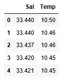
df> => pd.read_csv(> 'bottle.csv'> )> df_binary> => df[[> 'Salnty'> ,> 'T_degC'> ]]> > # Taking only the selected two attributes from the dataset> df_binary.columns> => [> 'Sal'> ,> 'Temp'> ]> #display the first 5 rows> df_binary.head()>

산출:

3단계: 데이터 분산 탐색

파이썬3

#plotting the Scatter plot to check relationship between Sal and Temp> sns.lmplot(x> => 'Sal'> , y> => 'Temp'> , data> => df_binary, order> => 2> , ci> => None> )> plt.show()>

산출:

4단계: 데이터 정리

파이썬3

# Eliminating NaN or missing input numbers> df_binary.fillna(method> => 'ffill'> , inplace> => True> )>

5단계: 모델 훈련

파이썬3

X> => np.array(df_binary[> 'Sal'> ]).reshape(> -> 1> ,> 1> )> y> => np.array(df_binary[> 'Temp'> ]).reshape(> -> 1> ,> 1> )> > # Separating the data into independent and dependent variables> # Converting each dataframe into a numpy array> # since each dataframe contains only one column> df_binary.dropna(inplace> => True> )> > # Dropping any rows with Nan values> X_train, X_test, y_train, y_test> => train_test_split(X, y, test_size> => 0.25> )> > # Splitting the data into training and testing data> regr> => LinearRegression()> > regr.fit(X_train, y_train)> print> (regr.score(X_test, y_test))>

산출:

6단계: 결과 탐색

파이썬3

y_pred> => regr.predict(X_test)> plt.scatter(X_test, y_test, color> => 'b'> )> plt.plot(X_test, y_pred, color> => 'k'> )> > plt.show()> # Data scatter of predicted values>

산출:

우리 모델의 낮은 정확도 점수는 회귀 모델이 기존 데이터에 잘 맞지 않음을 나타냅니다. 이는 우리 데이터가 선형 회귀 분석에 적합하지 않음을 나타냅니다. 그러나 때로는 데이터 세트의 일부만 고려하면 데이터 세트가 선형 회귀 분석을 허용할 수도 있습니다. 그 가능성을 확인해 보겠습니다.

7단계: 더 작은 데이터세트로 작업하기

파이썬3

df_binary500> => df_binary[:][:> 500> ]> > # Selecting the 1st 500 rows of the data> sns.lmplot(x> => 'Sal'> , y> => 'Temp'> , data> => df_binary500,> > order> => 2> , ci> => None> )>

산출:

처음 500개 행이 선형 모델을 따르는 것을 이미 볼 수 있습니다. 이전과 동일한 단계를 계속합니다.

파이썬3

df_binary500.fillna(method> => 'fill'> , inplace> => True> )> > X> => np.array(df_binary500[> 'Sal'> ]).reshape(> -> 1> ,> 1> )> y> => np.array(df_binary500[> 'Temp'> ]).reshape(> -> 1> ,> 1> )> > df_binary500.dropna(inplace> => True> )> X_train, X_test, y_train, y_test> => train_test_split(X, y, test_size> => 0.25> )> > regr> => LinearRegression()> regr.fit(X_train, y_train)> print> (regr.score(X_test, y_test))>

산출:

파이썬3

y_pred> => regr.predict(X_test)> plt.scatter(X_test, y_test, color> => 'b'> )> plt.plot(X_test, y_pred, color> => 'k'> )> > plt.show()>

산출:

8단계: 회귀에 대한 평가 지표

마지막으로 평가 지표를 사용하여 선형 회귀 모델의 성능을 확인합니다. 회귀 알고리즘의 경우 모델 성능을 확인하기 위해 평균_절대오류 및 평균제곱_오류 측정항목을 널리 사용합니다.

파이썬3

from> sklearn.metrics> import> mean_absolute_error,mean_squared_error> > mae> => mean_absolute_error(y_true> => y_test,y_pred> => y_pred)> #squared True returns MSE value, False returns RMSE value.> mse> => mean_squared_error(y_true> => y_test,y_pred> => y_pred)> #default=True> rmse> => mean_squared_error(y_true> => y_test,y_pred> => y_pred,squared> => False> )> > print> (> 'MAE:'> ,mae)> print> (> 'MSE:'> ,mse)> print> (> 'RMSE:'> ,rmse)>

산출:

MAE: 0.7927322046360309 MSE: 1.0251137190180517 RMSE: 1.0124789968281078