Šiame straipsnyje aptariami tiesinės regresijos pagrindai ir jos įgyvendinimas Python programavimo kalba. Tiesinė regresija yra statistinis metodas, skirtas modeliuoti ryšius tarp priklausomo kintamojo su tam tikra nepriklausomų kintamųjų rinkiniu.

Pastaba: Šiame straipsnyje mes vadiname priklausomus kintamuosius kaip atsakymus ir nepriklausomi kintamieji kaip funkcijos dėl paprastumo. Siekdami suteikti pagrindinį supratimą apie tiesinę regresiją, pradedame nuo paprasčiausios tiesinės regresijos versijos, t.y. Paprasta tiesinė regresija .

Kas yra tiesinė regresija?

Tiesinė regresija yra statistinis metodas, naudojamas prognozuoti nenutrūkstamą priklausomą kintamąjį (tikslinį kintamąjį), pagrįstą vienu ar daugiau nepriklausomų kintamųjų (numatomųjų kintamųjų). Šis metodas daro prielaidą, kad priklausomų ir nepriklausomų kintamųjų yra tiesinis ryšys, o tai reiškia, kad priklausomas kintamasis keičiasi proporcingai nepriklausomų kintamųjų pokyčiams. Kitaip tariant, tiesinė regresija naudojama norint nustatyti, kiek vienas ar keli kintamieji gali numatyti priklausomo kintamojo reikšmę.

Prielaidos, kurias darome tiesinės regresijos modelyje:

Toliau pateiktos pagrindinės prielaidos, kurias daro tiesinės regresijos modelis duomenų rinkiniui, kuriam jis taikomas:

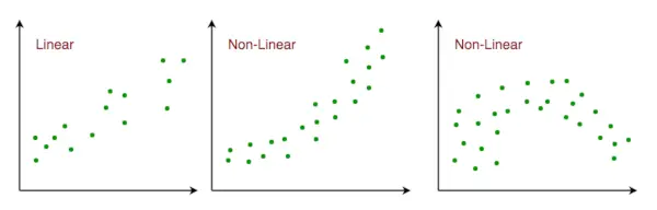
• Linijinis ryšys : Ryšys tarp atsako ir savybių kintamųjų turėtų būti tiesinis. Tiesiškumo prielaidą galima patikrinti naudojant sklaidos diagramas. Kaip parodyta toliau, 1 paveikslas rodo tiesiškai susijusius kintamuosius, o 2 ir 3 paveiksluose esantys kintamieji greičiausiai yra nelinijiniai. Taigi, 1 paveikslas suteiks geresnes prognozes naudojant tiesinę regresiją.

Linijinis ryšys i ypatybių erdvėje

• Mažas daugiakolineariškumas arba jo nėra : Daroma prielaida, kad duomenų daugiakolineariškumas yra mažas arba jo nėra. Daugiakolinisiškumas atsiranda tada, kai požymiai (arba nepriklausomi kintamieji) nėra nepriklausomi vienas nuo kito.
• Maža arba visai nėra autokoreliacijos : Daroma prielaida, kad autokoreliacijos duomenyse yra mažai arba visai nėra. Autokoreliacija atsiranda, kai liekamosios paklaidos nėra nepriklausomos viena nuo kitos. Norėdami gauti daugiau informacijos apie šią temą, galite kreiptis čia.
• Jokių nuokrypių: Manome, kad duomenyse nėra jokių nukrypimų. Nukrypimai yra duomenų taškai, kurie yra toli nuo kitų duomenų. Nukrypimai gali turėti įtakos analizės rezultatams.
• Homoscedastiškumas : Homoskedastiškumas apibūdina situaciją, kai klaidos terminas (ty triukšmas arba atsitiktinis trikdžių ryšys tarp nepriklausomų kintamųjų ir priklausomo kintamojo) yra vienodas visose nepriklausomų kintamųjų reikšmėse. Kaip parodyta toliau, 1 paveiksle yra homoskedastinis, o 2 paveiksle – heteroskedastinis.

Homoscedastiškumas tiesine regresija

Kai pasiekiame šio straipsnio pabaigą, toliau aptariame kai kuriuos tiesinės regresijos pritaikymus.

Tiesinės regresijos tipai

Yra du pagrindiniai tiesinės regresijos tipai:

• Paprasta tiesinė regresija: Tai apima priklausomo kintamojo prognozavimą, pagrįstą vienu nepriklausomu kintamuoju.
• Daugkartinė tiesinė regresija: Tai apima priklausomo kintamojo numatymą remiantis keliais nepriklausomais kintamaisiais.

Paprasta tiesinė regresija

Paprasta tiesinė regresija yra metodas prognozuoti a atsakymą naudojant a viena savybė . Tai vienas iš elementariausių mašininis mokymasis modeliai, apie kuriuos susipažįsta mašininio mokymosi entuziastas. Taikant tiesinę regresiją, darome prielaidą, kad du kintamieji, ty priklausomi ir nepriklausomi kintamieji, yra tiesiškai susiję. Todėl bandome rasti tiesinę funkciją, kuri kaip galima tiksliau nuspėtų atsako reikšmę (y) kaip funkcijos arba nepriklausomo kintamojo (x) funkciją. Panagrinėkime duomenų rinkinį, kuriame kiekvienos funkcijos x atsako reikšmė y:

Apskritai mes apibrėžiame:

x kaip ypatybių vektorius , ty x = [x_1, x_2, …., x_n],

ir taip atsako vektorius , ty y = [y_1, y_2, …., y_n]

dėl n stebėjimų (anksčiau pateiktame pavyzdyje n=10). Aukščiau pateikto duomenų rinkinio sklaidos diagrama atrodo taip:

Atsitiktinai sugeneruotų duomenų sklaidos diagrama

Dabar užduotis yra surasti a geriausiai tinkanti linija aukščiau pateiktoje sklaidos diagramoje, kad galėtume numatyti atsaką į bet kokias naujas ypatybių vertes. (t. y. x reikšmės duomenų rinkinyje nėra) Ši eilutė vadinama a regresijos linija . Regresijos linijos lygtis pavaizduota taip:

h(x_i) = eta _0 + eta_1x_i

Čia

• h(x_i) reiškia numatoma atsako vertė už i ^th stebėjimas.
• b_0 ir b_1 yra regresijos koeficientai ir reiškia y-pertrauka ir nuolydis atitinkamai regresijos tiesės.

Norėdami sukurti savo modelį, turime išmokti arba įvertinti regresijos koeficientų b_0 ir b_1 reikšmes. Ir įvertinę šiuos koeficientus, galime naudoti modelį atsakymams numatyti!
Šiame straipsnyje mes naudosime principą Mažiausi kvadratai .

Dabar apsvarstykite:

y_i = eta_0 + eta_1x_i + varepsilon_i = h(x_i) + varepsilon_i Rightarrow varepsilon_i = y_i -h(x_i)

Čia e_i yra a liekamoji klaida tame stebėjime. Taigi, mūsų tikslas yra sumažinti bendrą likutinę paklaidą. Kvadrato paklaidos arba sąnaudų funkciją J apibrėžiame kaip:

J(eta_0,eta_1)= frac{1}{2n} sum_{i=1}^{n} varepsilon_i^{2}

Ir mūsų užduotis yra rasti b reikšmę ₀ ir b ₁ kuriam J(g ₀ , b ₁ ) yra minimalus! Nesigilindami į matematines detales, rezultatą pateikiame čia:

eta_1 = frac{SS_{xy}}{SS_{xx}}

eta_0 = ar{y} – eta_1ar{x}

Kur SS _xy yra y ir x kryžminių nuokrypių suma:

SS_{xy} = sum_{i=1}^{n} (x_i-ar{x})(y_i-ar{y}) = sum_{i=1}^{n} y_ix_i – nar{x}ar{y}

Ir SS _xx yra x nuokrypių kvadratų suma:

SS_{xx} = sum_{i=1}^{n} (x_i-ar{x})^2 = sum_{i=1}^{n}x_i^2 – n(ar{x})^2

Python paprastos tiesinės regresijos įgyvendinimas

Mes galime naudoti Python kalba išmokti tiesinės regresijos modelių koeficientą. Norėdami nubraižyti įvesties duomenis ir geriausiai pritaikytą liniją, naudosime matplotlib biblioteka. Tai viena iš dažniausiai naudojamų Python bibliotekų grafikams braižyti. Štai paprastos tiesinės regresijos naudojant Python pavyzdys.

Bibliotekų importavimas

Python3

     Estimating Coefficients Function  This function, estimate_coef(), takes the input data x (independent variable) and y (dependent variable) and estimates the coefficients of the linear regression line using the least squares method.   Calculating Number of Observations:   n = np.size(x) determines the number of data points.  Calculating Means:   m_x = np.mean(x) and m_y = np.mean(y) compute the mean values of x and y, respectively.  Calculating Cross-Deviation and Deviation about x:   SS_xy = np.sum(y*x) - n*m_y*m_x and SS_xx = np.sum(x*x) - n*m_x*m_x calculate the sum of squared deviations between x and y and the sum of squared deviations of x about its mean, respectively.  Calculating Regression Coefficients:   b_1 = SS_xy / SS_xx and b_0 = m_y - b_1*m_x determine the slope (b_1) and intercept (b_0) of the regression line using the least squares method.  Returning Coefficients:   The function returns the estimated coefficients as a tuple (b_0, b_1). Python3         def estimate_coef(x, y):   # number of observations/points   n = np.size(x)     # mean of x and y vector   m_x = np.mean(x)   m_y = np.mean(y)     # calculating cross-deviation and deviation about x   SS_xy = np.sum(y*x) - n*m_y*m_x   SS_xx = np.sum(x*x) - n*m_x*m_x     # calculating regression coefficients   b_1 = SS_xy / SS_xx   b_0 = m_y - b_1*m_x     return (b_0, b_1)         Plotting Regression Line Function  This function, plot_regression_line(), takes the input data x (independent variable), y (dependent variable), and the estimated coefficients b to plot the regression line and the data points.   Plotting Scatter Plot:   plt.scatter(x, y, color = 'm', marker = 'o', s = 30) plots the original data points as a scatter plot with red markers.  Calculating Predicted Response Vector:   y_pred = b[0] + b[1]*x calculates the predicted values for y based on the estimated coefficients b.  Plotting Regression Line:   plt.plot(x, y_pred, color = 'g') plots the regression line using the predicted values and the independent variable x.  Adding Labels:   plt.xlabel('x') and plt.ylabel('y') label the x-axis as 'x' and the y-axis as 'y', respectively. Python3         def plot_regression_line(x, y, b):   # plotting the actual points as scatter plot   plt.scatter(x, y, color = 'm',   marker = 'o', s = 30)     # predicted response vector   y_pred = b[0] + b[1]*x     # plotting the regression line   plt.plot(x, y_pred, color = 'g')     # putting labels   plt.xlabel('x')   plt.ylabel('y')         Output:    Scatterplot of the points along with the regression line   Main Function  The provided code implements simple linear regression analysis by defining a function main() that performs the following steps:   Data Definition:   Defines the independent variable (x) and dependent variable (y) as NumPy arrays.  Coefficient Estimation:   Calls the estimate_coef() function to determine the coefficients of the linear regression line using the provided data.  Printing Coefficients:   Prints the estimated intercept (b_0) and slope (b_1) of the regression line. Python3         def main():   # observations / data   x = np.array([0, 1, 2, 3, 4, 5, 6, 7, 8, 9])   y = np.array([1, 3, 2, 5, 7, 8, 8, 9, 10, 12])     # estimating coefficients   b = estimate_coef(x, y)   print('Estimated coefficients:
b_0 = {}    
b_1 = {}'.format(b        Output:    Estimated coefficients: b_0 = -0.0586206896552 b_1 = 1.45747126437Multiple Linear RegressionMultiple linear regression attempts to model the relationship between   two or more features   and a response by fitting a linear equation to the observed data. Clearly, it is nothing but an extension of simple linear regression. Consider a dataset with   p   features(or independent variables) and one response(or dependent variable).  Also, the dataset contains   n   rows/observations.  We define: X (  feature matrix  ) = a matrix of size   n X p   where xij denotes the values of the jth feature for ith observation.  So,   and y (  response vector  ) = a vector of size   n   where y_{i} denotes the value of response for ith observation.   The   regression line   for   p   features is represented as:   where h(x_i) is   predicted response value   for ith observation and b_0, b_1, …, b_p are the   regression coefficients  . Also, we can write:   where e_i represents a   residual error   in ith observation. We can generalize our linear model a little bit more by representing feature matrix   X   as:   So now, the linear model can be expressed in terms of matrices as:   where,   and  Now, we determine an   estimate of b  , i.e. b’ using the   Least Squares method  . As already explained, the Least Squares method tends to determine b’ for which total residual error is minimized. We present the result directly here:   where ‘ represents the transpose of the matrix while -1 represents the  matrix inverse . Knowing the least square estimates, b’, the multiple linear regression model can now be estimated as:  where y’ is the   estimated response vector  .   Python Implementation of Multiple Linear Regression  For  multiple linear regression  using Python, we will use the Boston house pricing dataset.  Importing Libraries Python3         from sklearn.model_selection import train_test_split  import matplotlib.pyplot as plt  import numpy as np  from sklearn import datasets, linear_model, metrics  import pandas as pd         Loading the Boston Housing Dataset  The code downloads the Boston Housing dataset from the provided URL and reads it into a Pandas DataFrame (raw_df) Python3         data_url = ' http://lib.stat.cmu.edu/datasets/boston ' raw_df = pd.read_csv(data_url, sep='s+',   skiprows=22, header=None)        Preprocessing Data  This extracts the input variables (X) and target variable (y) from the DataFrame. The input variables are selected from every other row to match the target variable, which is available every other row. Python3         X = np.hstack([raw_df.values[::2, :],   raw_df.values[1::2, :2]])  y = raw_df.values[1::2, 2]        Splitting Data into Training and Testing Sets  Here it divides the data into training and testing sets using the train_test_split() function from scikit-learn. The test_size parameter specifies that 40% of the data should be used for testing. Python3         X_train, X_test,   y_train, y_test = train_test_split(X, y,   test_size=0.4,   random_state=1)        Creating and Training the Linear Regression Model  This initializes a LinearRegression object (reg) and trains the model using the training data (X_train, y_train) Python3         reg = linear_model.LinearRegression()  reg.fit(X_train, y_train)        Evaluating Model Performance  Evaluates the model’s performance by printing the regression coefficients and calculating the variance score, which measures the proportion of explained variance. A score of 1 indicates perfect prediction. Python3         # regression coefficients  print('Coefficients: ', reg.coef_)    # variance score: 1 means perfect prediction  print('Variance score: {}'.format(reg.score(X_test, y_test)))        Output:    Coefficients: [ -8.80740828e-02 6.72507352e-02 5.10280463e-02 2.18879172e+00 -1.72283734e+01 3.62985243e+00 2.13933641e-03 -1.36531300e+00 2.88788067e-01 -1.22618657e-02 -8.36014969e-01 9.53058061e-03 -5.05036163e-01] Variance score: 0.720898784611  Plotting Residual Errors   Plotting and analyzing the residual errors, which represent the difference between the predicted values and the actual values. Python3         # plot for residual error    # setting plot style  plt.style.use('fivethirtyeight')    # plotting residual errors in training data  plt.scatter(reg.predict(X_train),   reg.predict(X_train) - y_train,   color='green', s=10,   label='Train data')    # plotting residual errors in test data  plt.scatter(reg.predict(X_test),   reg.predict(X_test) - y_test,   color='blue', s=10,   label='Test data')    # plotting line for zero residual error  plt.hlines(y=0, xmin=0, xmax=50, linewidth=2)    # plotting legend  plt.legend(loc='upper right')    # plot title  plt.title('Residual errors')    # method call for showing the plot  plt.show()         Output:    Residual Error Plot for the Multiple Linear Regression In the above example, we determine the accuracy score using   Explained Variance Score  . We define:  explained_variance_score = 1 – Var{y – y’}/Var{y}  where y’ is the estimated target output, y is the corresponding (correct) target output, and Var is Variance, the square of the standard deviation. The best possible score is 1.0, lower values are worse. Polynomial Linear Regression  Polynomial Regression   is a form of linear regression in which the relationship between the independent variable x and dependent variable y is modeled as an   nth-degree   polynomial. Polynomial regression fits a nonlinear relationship between the value of x and the corresponding conditional mean of y, denoted E(y | x).   Choosing a Degree for Polynomial Regression  The choice of degree for polynomial regression is a trade-off between bias and variance. Bias is the tendency of a model to consistently predict the same value, regardless of the true value of the dependent variable. Variance is the tendency of a model to make different predictions for the same data point, depending on the specific training data used. A higher-degree polynomial can reduce bias but can also increase variance, leading to overfitting. Conversely, a lower-degree polynomial can reduce variance but can also increase bias. There are a number of methods for choosing a degree for polynomial regression, such as cross-validation and using information criteria such as Akaike information criterion (AIC) or Bayesian information criterion (BIC). Implementation of Polynomial Regression using Python Implementing the Polynomial regression using Python: Here we will import all the necessary libraries for data analysis and machine learning tasks and then loads the ‘Position_Salaries.csv’ dataset using Pandas. It then prepares the data for modeling by handling missing values and encoding categorical data. Finally, it splits the data into training and testing sets and standardizes the numerical features using StandardScaler. Python3         import pandas as pd  import matplotlib.pyplot as plt  import seaborn as sns  import sklearn  import warnings    from sklearn.preprocessing import LabelEncoder  from sklearn.impute import KNNImputer  from sklearn.model_selection import train_test_split  from sklearn.preprocessing import StandardScaler  from sklearn.metrics import f1_score  from sklearn.ensemble import RandomForestRegressor  from sklearn.ensemble import RandomForestRegressor  from sklearn.model_selection import cross_val_score    warnings.filterwarnings('ignore')    df = pd.read_csv('Position_Salaries.csv')    X = df.iloc[:,1:2].values  y = df.iloc[:,2].values  x        Output:   array([[ 1, 45000, 0], [ 2, 50000, 4], [ 3, 60000, 8], [ 4, 80000, 5], [ 5, 110000, 3], [ 6, 150000, 7], [ 7, 200000, 6], [ 8, 300000, 9], [ 9, 500000, 1], [ 10, 1000000, 2]], dtype=int64) The code creates a linear regression model and fits it to the provided data, establishing a linear relationship between the independent and dependent variables. Python3         from sklearn.linear_model import LinearRegression  lin_reg=LinearRegression()  lin_reg.fit(X,y)      The code performs quadratic and cubic regression by generating polynomial features from the original data and fitting linear regression models to these features. This enables modeling nonlinear relationships between the independent and dependent variables. Python3         from sklearn.preprocessing import PolynomialFeatures  poly_reg2=PolynomialFeatures(degree=2)  X_poly=poly_reg2.fit_transform(X)  lin_reg_2=LinearRegression()  lin_reg_2.fit(X_poly,y)    poly_reg3=PolynomialFeatures(degree=3)  X_poly3=poly_reg3.fit_transform(X)  lin_reg_3=LinearRegression()  lin_reg_3.fit(X_poly3,y)      The code creates a scatter plot of the data point, It effectively visualizes the linear relationship between position level and salary. Python3         plt.scatter(X,y,color='red')  plt.plot(X,lin_reg.predict(X),color='green')  plt.title('Simple Linear Regression')  plt.xlabel('Position Level')  plt.ylabel('Salary')  plt.show()        Output:    The code creates a scatter plot of the data points, overlays the predicted quadratic and cubic regression lines. It effectively visualizes the nonlinear relationship between position level and salary and compares the fits of quadratic and cubic regression models. Python3         plt.style.use('fivethirtyeight')  plt.scatter(X,y,color='red')  plt.plot(X,lin_reg_2.predict(poly_reg2.fit_transform(X)),color='green')  plt.plot(X,lin_reg_3.predict(poly_reg3.fit_transform(X)),color='yellow')  plt.title('Polynomial Linear Regression Degree 2')  plt.xlabel('Position Level')  plt.ylabel('Salary')  plt.show()        Output:    The code effectively visualizes the relationship between position level and salary using cubic regression and generates a continuous prediction line for a broader range of position levels. Python3         plt.style.use('fivethirtyeight')  X_grid=np.arange(min(X),max(X),0.1) # This will give us a vector.We will have to convert this into a matrix  X_grid=X_grid.reshape((len(X_grid),1))  plt.scatter(X,y,color='red')  plt.plot(X_grid,lin_reg_3.predict(poly_reg3.fit_transform(X_grid)),color='lightgreen')    #plt.plot(X,lin_reg_3.predict(poly_reg3.fit_transform(X)),color='green')  plt.title('Polynomial Linear Regression Degree 3')  plt.xlabel('Position Level')  plt.ylabel('Salary')  plt.show()        Output:    Applications of Linear Regression  Trend lines:   A trend line represents the variation in quantitative data with the passage of time (like GDP, oil prices, etc.). These trends usually follow a linear relationship. Hence, linear regression can be applied to predict future values. However, this method suffers from a lack of scientific validity in cases where other potential changes can affect the data.  Economics:   Linear regression is the predominant empirical tool in economics. For example, it is used to predict consumer spending, fixed investment spending, inventory investment, purchases of a country’s exports, spending on imports, the demand to hold liquid assets, labor demand, and labor supply.  Finance:   The capital price asset model uses linear regression to analyze and quantify the systematic risks of an investment.  Biology:   Linear regression is used to model causal relationships between parameters in biological systems.  Advantages   of Linear Regression  Easy to interpret:   The coefficients of a linear regression model represent the change in the dependent variable for a one-unit change in the independent variable, making it simple to comprehend the relationship between the variables.  Robust to outliers:   Linear regression is relatively robust to outliers meaning it is less affected by extreme values of the independent variable compared to other statistical methods.  Can handle both linear and nonlinear relationships:   Linear regression can be used to model both linear and nonlinear relationships between variables. This is because the independent variable can be transformed before it is used in the model.  No need for feature scaling or transformation:   Unlike some machine learning algorithms, linear regression does not require feature scaling or transformation. This can be a significant advantage, especially when dealing with large datasets.  Disadvantages   of Linear Regression  Assumes linearity:   Linear regression assumes that the relationship between the independent variable and the dependent variable is linear. This assumption may not be valid for all data sets. In cases where the relationship is nonlinear, linear regression may not be a good choice.  Sensitive to multicollinearity:   Linear regression is sensitive to multicollinearity. This occurs when there is a high correlation between the independent variables. Multicollinearity can make it difficult to interpret the coefficients of the model and can lead to overfitting.  May not be suitable for highly complex relationships:   Linear regression may not be suitable for modeling highly complex relationships between variables. For example, it may not be able to model relationships that include interactions between the independent variables.  Not suitable for classification tasks:   Linear regression is a regression algorithm and is not suitable for classification tasks, which involve predicting a categorical variable rather than a continuous variable.Frequently Asked Question(FAQs)1.   How to use linear regression to make predictions?  Once a linear regression model has been trained, it can be used to make predictions for new data points. The scikit-learn LinearRegression class provides a method called predict() that can be used to make predictions. 2.  What is linear regression?  Linear regression is a supervised machine learning algorithm used to predict a continuous numerical output. It assumes that the relationship between the independent variables (features) and the dependent variable (target) is linear, meaning that the predicted value of the target can be calculated as a linear combination of the features.   3. How to perform linear regression in Python?  There are several libraries in Python that can be used to perform linear regression, including scikit-learn, statsmodels, and NumPy. The scikit-learn library is the most popular choice for machine learning tasks, and it provides a simple and efficient implementation of linear regression. 4.   What are some applications of linear regression?  Linear regression is a versatile algorithm that can be used for a wide variety of applications, including finance, healthcare, and marketing. Some specific examples include: Predicting house pricesPredicting stock pricesDiagnosing medical conditionsPredicting customer churn5. How linear regression is implemented in sklearn?Linear regression is implemented in scikit-learn using the LinearRegression class. This class provides methods to fit a linear regression model to a training dataset and predict the target value for new data points.