Regresión lineal (implementación de Python)
Este artículo analiza los conceptos básicos de la regresión lineal y su implementación en el lenguaje de programación Python. La regresión lineal es un método estadístico para modelar relaciones entre una variable dependiente con un conjunto determinado de variables independientes.
Nota: En este artículo nos referimos a las variables dependientes como respuestas y variables independientes como características por simplicidad. Para proporcionar una comprensión básica de la regresión lineal, comenzamos con la versión más básica de la regresión lineal, es decir Regresión lineal simple .
¿Qué es la regresión lineal?
Regresión lineal es un método estadístico que se utiliza para predecir una variable dependiente continua (variable objetivo) en función de una o más variables independientes (variables predictivas). Esta técnica supone una relación lineal entre las variables dependientes e independientes, lo que implica que la variable dependiente cambia proporcionalmente con los cambios en las variables independientes. En otras palabras, la regresión lineal se utiliza para determinar hasta qué punto una o más variables pueden predecir el valor de la variable dependiente.
Suposiciones que hacemos en un modelo de regresión lineal:
A continuación se detallan los supuestos básicos que hace un modelo de regresión lineal con respecto al conjunto de datos al que se aplica:
- Relación lineal : La relación entre las variables de respuesta y características debe ser lineal. El supuesto de linealidad se puede probar mediante diagramas de dispersión. Como se muestra a continuación, la primera figura representa variables relacionadas linealmente, mientras que las variables de la segunda y tercera figuras probablemente no sean lineales. Entonces, la primera figura dará mejores predicciones utilizando la regresión lineal.

Relación lineal en el espacio de características.
- Poca o nula multicolinealidad : Se supone que hay poca o ninguna multicolinealidad en los datos. La multicolinealidad ocurre cuando las características (o variables independientes) no son independientes entre sí.
- Poca o nula autocorrelación : Otro supuesto es que hay poca o ninguna autocorrelación en los datos. La autocorrelación ocurre cuando los errores residuales no son independientes entre sí. Puede consultar aquí para obtener más información sobre este tema.
- Sin valores atípicos: Suponemos que no hay valores atípicos en los datos. Los valores atípicos son puntos de datos que están lejos del resto de los datos. Los valores atípicos pueden afectar los resultados del análisis.
- homocedasticidad : La homocedasticidad describe una situación en la que el término de error (es decir, el ruido o perturbación aleatoria en la relación entre las variables independientes y la variable dependiente) es el mismo en todos los valores de las variables independientes. Como se muestra a continuación, la figura 1 tiene homocedasticidad mientras que la Figura 2 tiene heterocedasticidad.

Homoscedasticidad en regresión lineal
Al llegar al final de este artículo, analizamos algunas aplicaciones de la regresión lineal a continuación.
Tipos de regresión lineal
Hay dos tipos principales de regresión lineal:
- Regresión lineal simple: Esto implica predecir una variable dependiente basándose en una única variable independiente.
- Regresión lineal múltiple: Esto implica predecir una variable dependiente basándose en múltiples variables independientes.
Regresión lineal simple
Simple regresión lineal es un método para predecir una respuesta usando un característica única . Es uno de los más básicos. aprendizaje automático Modelos que un entusiasta del aprendizaje automático conoce. En la regresión lineal, asumimos que las dos variables, es decir, las variables dependientes e independientes, están relacionadas linealmente. Por lo tanto, tratamos de encontrar una función lineal que prediga el valor de respuesta (y) con la mayor precisión posible como función de la característica o variable independiente (x). Consideremos un conjunto de datos donde tenemos un valor de respuesta y para cada característica x:

Por generalidad, definimos:
x como vector de caracteristicas , es decir x = [x_1, x_2,…., x_n],
y as vector de respuesta , i.e y = [y_1, y_2, …., y_n]
para norte observaciones (en el ejemplo anterior, n=10). Un diagrama de dispersión del conjunto de datos anterior se ve así:

Diagrama de dispersión para los datos generados aleatoriamente.
Ahora la tarea es encontrar un línea que mejor se adapta en el diagrama de dispersión anterior para que podamos predecir la respuesta para cualquier valor de característica nueva. (es decir, un valor de x que no está presente en un conjunto de datos) Esta línea se llama línea de regresión . La ecuación de la recta de regresión se representa como:
Aquí,
- h(x_i) representa el valor de respuesta previsto para yo th observación.
- b_0 y b_1 son coeficientes de regresión y representan la y-intercept y pendiente de la línea de regresión respectivamente.
Para crear nuestro modelo, debemos aprender o estimar los valores de los coeficientes de regresión b_0 y b_1. Y una vez que hayamos estimado estos coeficientes, ¡podemos usar el modelo para predecir respuestas!
En este artículo vamos a utilizar el principio de Mínimos cuadrados .
Ahora considere:
Aquí, e_i es un error residual en su observación. Entonces, nuestro objetivo es minimizar el error residual total. Definimos el error al cuadrado o función de costo, J como:
Y nuestra tarea es encontrar el valor de b. 0 y B 1 para lo cual J(b 0 , b 1 ) es mínimo! Sin entrar en detalles matemáticos, presentamos aquí el resultado:
donde SS xy es la suma de las desviaciones cruzadas de y y x:
y SS xx es la suma de las desviaciones al cuadrado de x:
Implementación en Python de regresión lineal simple
Podemos usar el Pitón Lenguaje para aprender el coeficiente de modelos de regresión lineal. Para trazar los datos de entrada y la línea mejor ajustada usaremos el matplotlib biblioteca. Es una de las bibliotecas de Python más utilizadas para trazar gráficos. Aquí está el ejemplo de regresión lineal simple usando Python.
Importación de bibliotecas
Python3
import> numpy as np> import> matplotlib.pyplot as plt> |
     Estimating Coefficients Function  This function, estimate_coef(), takes the input data x (independent variable) and y (dependent variable) and estimates the coefficients of the linear regression line using the least squares method.   Calculating Number of Observations:   n = np.size(x) determines the number of data points.  Calculating Means:   m_x = np.mean(x) and m_y = np.mean(y) compute the mean values of x and y, respectively.  Calculating Cross-Deviation and Deviation about x:   SS_xy = np.sum(y*x) - n*m_y*m_x and SS_xx = np.sum(x*x) - n*m_x*m_x calculate the sum of squared deviations between x and y and the sum of squared deviations of x about its mean, respectively.  Calculating Regression Coefficients:   b_1 = SS_xy / SS_xx and b_0 = m_y - b_1*m_x determine the slope (b_1) and intercept (b_0) of the regression line using the least squares method.  Returning Coefficients:   The function returns the estimated coefficients as a tuple (b_0, b_1). Python3         def estimate_coef(x, y):   # number of observations/points   n = np.size(x)     # mean of x and y vector   m_x = np.mean(x)   m_y = np.mean(y)     # calculating cross-deviation and deviation about x   SS_xy = np.sum(y*x) - n*m_y*m_x   SS_xx = np.sum(x*x) - n*m_x*m_x     # calculating regression coefficients   b_1 = SS_xy / SS_xx   b_0 = m_y - b_1*m_x     return (b_0, b_1)         Plotting Regression Line Function  This function, plot_regression_line(), takes the input data x (independent variable), y (dependent variable), and the estimated coefficients b to plot the regression line and the data points.   Plotting Scatter Plot:   plt.scatter(x, y, color = 'm', marker = 'o', s = 30) plots the original data points as a scatter plot with red markers.  Calculating Predicted Response Vector:   y_pred = b[0] + b[1]*x calculates the predicted values for y based on the estimated coefficients b.  Plotting Regression Line:   plt.plot(x, y_pred, color = 'g') plots the regression line using the predicted values and the independent variable x.  Adding Labels:   plt.xlabel('x') and plt.ylabel('y') label the x-axis as 'x' and the y-axis as 'y', respectively. Python3         def plot_regression_line(x, y, b):   # plotting the actual points as scatter plot   plt.scatter(x, y, color = 'm',   marker = 'o', s = 30)     # predicted response vector   y_pred = b[0] + b[1]*x     # plotting the regression line   plt.plot(x, y_pred, color = 'g')     # putting labels   plt.xlabel('x')   plt.ylabel('y')         Output:    Scatterplot of the points along with the regression line   Main Function  The provided code implements simple linear regression analysis by defining a function main() that performs the following steps:   Data Definition:   Defines the independent variable (x) and dependent variable (y) as NumPy arrays.  Coefficient Estimation:   Calls the estimate_coef() function to determine the coefficients of the linear regression line using the provided data.  Printing Coefficients:   Prints the estimated intercept (b_0) and slope (b_1) of the regression line. Python3         def main():   # observations / data   x = np.array([0, 1, 2, 3, 4, 5, 6, 7, 8, 9])   y = np.array([1, 3, 2, 5, 7, 8, 8, 9, 10, 12])     # estimating coefficients   b = estimate_coef(x, y)   print('Estimated coefficients:
b_0 = {}
b_1 = {}'.format(b        Output:    Estimated coefficients: b_0 = -0.0586206896552 b_1 = 1.45747126437Multiple Linear RegressionMultiple linear regression attempts to model the relationship between   two or more features   and a response by fitting a linear equation to the observed data. Clearly, it is nothing but an extension of simple linear regression. Consider a dataset with   p   features(or independent variables) and one response(or dependent variable).  Also, the dataset contains   n   rows/observations.  We define: X (  feature matrix  ) = a matrix of size   n X p   where xij denotes the values of the jth feature for ith observation.  So,   and y (  response vector  ) = a vector of size   n   where y_{i} denotes the value of response for ith observation.   The   regression line   for   p   features is represented as:   where h(x_i) is   predicted response value   for ith observation and b_0, b_1, …, b_p are the   regression coefficients  . Also, we can write:   where e_i represents a   residual error   in ith observation. We can generalize our linear model a little bit more by representing feature matrix   X   as:   So now, the linear model can be expressed in terms of matrices as:   where,   and  Now, we determine an   estimate of b  , i.e. b’ using the   Least Squares method  . As already explained, the Least Squares method tends to determine b’ for which total residual error is minimized. We present the result directly here:   where ‘ represents the transpose of the matrix while -1 represents the  matrix inverse . Knowing the least square estimates, b’, the multiple linear regression model can now be estimated as:  where y’ is the   estimated response vector  .   Python Implementation of Multiple Linear Regression  For  multiple linear regression  using Python, we will use the Boston house pricing dataset.  Importing Libraries Python3         from sklearn.model_selection import train_test_split  import matplotlib.pyplot as plt  import numpy as np  from sklearn import datasets, linear_model, metrics  import pandas as pd         Loading the Boston Housing Dataset  The code downloads the Boston Housing dataset from the provided URL and reads it into a Pandas DataFrame (raw_df) Python3         data_url = ' http://lib.stat.cmu.edu/datasets/boston ' raw_df = pd.read_csv(data_url, sep='s+',   skiprows=22, header=None)        Preprocessing Data  This extracts the input variables (X) and target variable (y) from the DataFrame. The input variables are selected from every other row to match the target variable, which is available every other row. Python3         X = np.hstack([raw_df.values[::2, :],   raw_df.values[1::2, :2]])  y = raw_df.values[1::2, 2]        Splitting Data into Training and Testing Sets  Here it divides the data into training and testing sets using the train_test_split() function from scikit-learn. The test_size parameter specifies that 40% of the data should be used for testing. Python3         X_train, X_test,   y_train, y_test = train_test_split(X, y,   test_size=0.4,   random_state=1)        Creating and Training the Linear Regression Model  This initializes a LinearRegression object (reg) and trains the model using the training data (X_train, y_train) Python3         reg = linear_model.LinearRegression()  reg.fit(X_train, y_train)        Evaluating Model Performance  Evaluates the model’s performance by printing the regression coefficients and calculating the variance score, which measures the proportion of explained variance. A score of 1 indicates perfect prediction. Python3         # regression coefficients  print('Coefficients: ', reg.coef_)    # variance score: 1 means perfect prediction  print('Variance score: {}'.format(reg.score(X_test, y_test)))        Output:    Coefficients: [ -8.80740828e-02 6.72507352e-02 5.10280463e-02 2.18879172e+00 -1.72283734e+01 3.62985243e+00 2.13933641e-03 -1.36531300e+00 2.88788067e-01 -1.22618657e-02 -8.36014969e-01 9.53058061e-03 -5.05036163e-01] Variance score: 0.720898784611  Plotting Residual Errors   Plotting and analyzing the residual errors, which represent the difference between the predicted values and the actual values. Python3         # plot for residual error    # setting plot style  plt.style.use('fivethirtyeight')    # plotting residual errors in training data  plt.scatter(reg.predict(X_train),   reg.predict(X_train) - y_train,   color='green', s=10,   label='Train data')    # plotting residual errors in test data  plt.scatter(reg.predict(X_test),   reg.predict(X_test) - y_test,   color='blue', s=10,   label='Test data')    # plotting line for zero residual error  plt.hlines(y=0, xmin=0, xmax=50, linewidth=2)    # plotting legend  plt.legend(loc='upper right')    # plot title  plt.title('Residual errors')    # method call for showing the plot  plt.show()         Output:    Residual Error Plot for the Multiple Linear Regression In the above example, we determine the accuracy score using   Explained Variance Score  . We define:  explained_variance_score = 1 – Var{y – y’}/Var{y}  where y’ is the estimated target output, y is the corresponding (correct) target output, and Var is Variance, the square of the standard deviation. The best possible score is 1.0, lower values are worse. Polynomial Linear Regression  Polynomial Regression   is a form of linear regression in which the relationship between the independent variable x and dependent variable y is modeled as an   nth-degree   polynomial. Polynomial regression fits a nonlinear relationship between the value of x and the corresponding conditional mean of y, denoted E(y | x).   Choosing a Degree for Polynomial Regression  The choice of degree for polynomial regression is a trade-off between bias and variance. Bias is the tendency of a model to consistently predict the same value, regardless of the true value of the dependent variable. Variance is the tendency of a model to make different predictions for the same data point, depending on the specific training data used. A higher-degree polynomial can reduce bias but can also increase variance, leading to overfitting. Conversely, a lower-degree polynomial can reduce variance but can also increase bias. There are a number of methods for choosing a degree for polynomial regression, such as cross-validation and using information criteria such as Akaike information criterion (AIC) or Bayesian information criterion (BIC). Implementation of Polynomial Regression using Python Implementing the Polynomial regression using Python: Here we will import all the necessary libraries for data analysis and machine learning tasks and then loads the ‘Position_Salaries.csv’ dataset using Pandas. It then prepares the data for modeling by handling missing values and encoding categorical data. Finally, it splits the data into training and testing sets and standardizes the numerical features using StandardScaler. Python3         import pandas as pd  import matplotlib.pyplot as plt  import seaborn as sns  import sklearn  import warnings    from sklearn.preprocessing import LabelEncoder  from sklearn.impute import KNNImputer  from sklearn.model_selection import train_test_split  from sklearn.preprocessing import StandardScaler  from sklearn.metrics import f1_score  from sklearn.ensemble import RandomForestRegressor  from sklearn.ensemble import RandomForestRegressor  from sklearn.model_selection import cross_val_score    warnings.filterwarnings('ignore')    df = pd.read_csv('Position_Salaries.csv')    X = df.iloc[:,1:2].values  y = df.iloc[:,2].values  x        Output:   array([[ 1, 45000, 0], [ 2, 50000, 4], [ 3, 60000, 8], [ 4, 80000, 5], [ 5, 110000, 3], [ 6, 150000, 7], [ 7, 200000, 6], [ 8, 300000, 9], [ 9, 500000, 1], [ 10, 1000000, 2]], dtype=int64) The code creates a linear regression model and fits it to the provided data, establishing a linear relationship between the independent and dependent variables. Python3         from sklearn.linear_model import LinearRegression  lin_reg=LinearRegression()  lin_reg.fit(X,y)      The code performs quadratic and cubic regression by generating polynomial features from the original data and fitting linear regression models to these features. This enables modeling nonlinear relationships between the independent and dependent variables. Python3         from sklearn.preprocessing import PolynomialFeatures  poly_reg2=PolynomialFeatures(degree=2)  X_poly=poly_reg2.fit_transform(X)  lin_reg_2=LinearRegression()  lin_reg_2.fit(X_poly,y)    poly_reg3=PolynomialFeatures(degree=3)  X_poly3=poly_reg3.fit_transform(X)  lin_reg_3=LinearRegression()  lin_reg_3.fit(X_poly3,y)      The code creates a scatter plot of the data point, It effectively visualizes the linear relationship between position level and salary. Python3         plt.scatter(X,y,color='red')  plt.plot(X,lin_reg.predict(X),color='green')  plt.title('Simple Linear Regression')  plt.xlabel('Position Level')  plt.ylabel('Salary')  plt.show()        Output:    The code creates a scatter plot of the data points, overlays the predicted quadratic and cubic regression lines. It effectively visualizes the nonlinear relationship between position level and salary and compares the fits of quadratic and cubic regression models. Python3         plt.style.use('fivethirtyeight')  plt.scatter(X,y,color='red')  plt.plot(X,lin_reg_2.predict(poly_reg2.fit_transform(X)),color='green')  plt.plot(X,lin_reg_3.predict(poly_reg3.fit_transform(X)),color='yellow')  plt.title('Polynomial Linear Regression Degree 2')  plt.xlabel('Position Level')  plt.ylabel('Salary')  plt.show()        Output:    The code effectively visualizes the relationship between position level and salary using cubic regression and generates a continuous prediction line for a broader range of position levels. Python3         plt.style.use('fivethirtyeight')  X_grid=np.arange(min(X),max(X),0.1) # This will give us a vector.We will have to convert this into a matrix  X_grid=X_grid.reshape((len(X_grid),1))  plt.scatter(X,y,color='red')  plt.plot(X_grid,lin_reg_3.predict(poly_reg3.fit_transform(X_grid)),color='lightgreen')    #plt.plot(X,lin_reg_3.predict(poly_reg3.fit_transform(X)),color='green')  plt.title('Polynomial Linear Regression Degree 3')  plt.xlabel('Position Level')  plt.ylabel('Salary')  plt.show()        Output:    Applications of Linear Regression  Trend lines:   A trend line represents the variation in quantitative data with the passage of time (like GDP, oil prices, etc.). These trends usually follow a linear relationship. Hence, linear regression can be applied to predict future values. However, this method suffers from a lack of scientific validity in cases where other potential changes can affect the data.  Economics:   Linear regression is the predominant empirical tool in economics. For example, it is used to predict consumer spending, fixed investment spending, inventory investment, purchases of a country’s exports, spending on imports, the demand to hold liquid assets, labor demand, and labor supply.  Finance:   The capital price asset model uses linear regression to analyze and quantify the systematic risks of an investment.  Biology:   Linear regression is used to model causal relationships between parameters in biological systems.  Advantages   of Linear Regression  Easy to interpret:   The coefficients of a linear regression model represent the change in the dependent variable for a one-unit change in the independent variable, making it simple to comprehend the relationship between the variables.  Robust to outliers:   Linear regression is relatively robust to outliers meaning it is less affected by extreme values of the independent variable compared to other statistical methods.  Can handle both linear and nonlinear relationships:   Linear regression can be used to model both linear and nonlinear relationships between variables. This is because the independent variable can be transformed before it is used in the model.  No need for feature scaling or transformation:   Unlike some machine learning algorithms, linear regression does not require feature scaling or transformation. This can be a significant advantage, especially when dealing with large datasets.  Disadvantages   of Linear Regression  Assumes linearity:   Linear regression assumes that the relationship between the independent variable and the dependent variable is linear. This assumption may not be valid for all data sets. In cases where the relationship is nonlinear, linear regression may not be a good choice.  Sensitive to multicollinearity:   Linear regression is sensitive to multicollinearity. This occurs when there is a high correlation between the independent variables. Multicollinearity can make it difficult to interpret the coefficients of the model and can lead to overfitting.  May not be suitable for highly complex relationships:   Linear regression may not be suitable for modeling highly complex relationships between variables. For example, it may not be able to model relationships that include interactions between the independent variables.  Not suitable for classification tasks:   Linear regression is a regression algorithm and is not suitable for classification tasks, which involve predicting a categorical variable rather than a continuous variable.Frequently Asked Question(FAQs)1.   How to use linear regression to make predictions?  Once a linear regression model has been trained, it can be used to make predictions for new data points. The scikit-learn LinearRegression class provides a method called predict() that can be used to make predictions. 2.  What is linear regression?  Linear regression is a supervised machine learning algorithm used to predict a continuous numerical output. It assumes that the relationship between the independent variables (features) and the dependent variable (target) is linear, meaning that the predicted value of the target can be calculated as a linear combination of the features.   3. How to perform linear regression in Python?  There are several libraries in Python that can be used to perform linear regression, including scikit-learn, statsmodels, and NumPy. The scikit-learn library is the most popular choice for machine learning tasks, and it provides a simple and efficient implementation of linear regression. 4.   What are some applications of linear regression?  Linear regression is a versatile algorithm that can be used for a wide variety of applications, including finance, healthcare, and marketing. Some specific examples include: Predicting house pricesPredicting stock pricesDiagnosing medical conditionsPredicting customer churn5. How linear regression is implemented in sklearn?Linear regression is implemented in scikit-learn using the LinearRegression class. This class provides methods to fit a linear regression model to a training dataset and predict the target value for new data points.