np.vstack: Для укладання масивів уздовж вертикальної осі. np.hstack: Для укладання масивів уздовж горизонтальної осі. np.column_stack: Щоб укласти одновимірні масиви як стовпці в двовимірні масиви. np.concatenate: Щоб укласти масиви вздовж вказаної осі (вісь передається як аргумент).

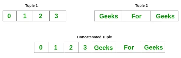
   import   numpy   as   np   a   =   np  .  array  ([[  1     2  ]   [  3     4  ]])   b   =   np  .  array  ([[  5     6  ]   [  7     8  ]])   # vertical stacking   print  (  'Vertical stacking:  n  '     np  .  vstack  ((  a     b  )))   # horizontal stacking   print  (  '  n  Horizontal stacking:  n  '     np  .  hstack  ((  a     b  )))   c   =   [  5     6  ]   # stacking columns   print  (  '  n  Column stacking:  n  '     np  .  column_stack  ((  a     c  )))   # concatenation method    print  (  '  n  Concatenating to 2nd axis:  n  '     np  .  concatenate  ((  a     b  )   1  ))   

Vertical stacking: [[1 2] [3 4] [5 6] [7 8]] Horizontal stacking: [[1 2 5 6] [3 4 7 8]] Column stacking: [[1 2 5] [3 4 6]] Concatenating to 2nd axis: [[1 2 5 6] [3 4 7 8]] 

np.hsplit: Розбити масив уздовж горизонтальної осі. np.vsplit: Розбити масив по вертикальній осі. np.array_split: Розбити масив уздовж вказаної осі.

   import   numpy   as   np   a   =   np  .  array  ([[  1     3     5     7     9     11  ]   [  2     4     6     8     10     12  ]])   # horizontal splitting   print  (  'Splitting along horizontal axis into 2 parts:  n  '     np  .  hsplit  (  a     2  ))   # vertical splitting   print  (  '  n  Splitting along vertical axis into 2 parts:  n  '     np  .  vsplit  (  a     2  ))   

Splitting along horizontal axis into 2 parts: [array([[1 3 5] [2 4 6]]) array([[ 7 9 11] [ 8 10 12]])] Splitting along vertical axis into 2 parts: [array([[ 1 3 5 7 9 11]]) array([[ 2 4 6 8 10 12]])] 

 A(2-D array): 4 x 3 B(1-D array): 3 Result : 4 x 3    
 A(4-D array): 7 x 1 x 6 x 1 B(3-D array): 3 x 1 x 5 Result : 7 x 3 x 6 x 5   But this would be a mismatch:  
 A: 4 x 3 B: 4   The simplest broadcasting example occurs when an array and a scalar value are combined in an operation. Consider the example given below: Python   
   import   numpy   as   np   a   =   np  .  array  ([  1.0     2.0     3.0  ])   # Example 1   b   =   2.0   print  (  a   *   b  )   # Example 2   c   =   [  2.0     2.0     2.0  ]   print  (  a   *   c  )   
  Output:  
[ 2. 4. 6.] [ 2. 4. 6.] 
 We can think of the scalar b being stretched during the arithmetic operation into an array with the same shape as a. The new elements in b as shown in above figure are simply copies of the original scalar. Although the stretching analogy is only conceptual. Numpy is smart enough to use the original scalar value without actually making copies so that broadcasting operations are as memory and computationally efficient as possible. Because Example 1 moves less memory (b is a scalar not an array) around during the multiplication it is about 10% faster than Example 2 using the standard numpy on Windows 2000 with one million element arrays! The figure below makes the concept more clear:    In above example the scalar b is stretched to become an array of with the same shape as a so the shapes are compatible for element-by-element multiplication. Now let us see an example where both arrays get stretched. Python   
   import   numpy   as   np   a   =   np  .  array  ([  0.0     10.0     20.0     30.0  ])   b   =   np  .  array  ([  0.0     1.0     2.0  ])   print  (  a  [:   np  .  newaxis  ]   +   b  )   
  Output:  
[[ 0. 1. 2.] [ 10. 11. 12.] [ 20. 21. 22.] [ 30. 31. 32.]]  
   У деяких випадках трансляція розтягує обидва масиви, щоб сформувати вихідний масив, більший за будь-який із початкових масивів.    Робота з датою і часом:   Numpy has core array data types which natively support datetime functionality. The data type is called datetime64 so named because datetime is already taken by the datetime library included in Python. Consider the example below for some examples: Python   
   import   numpy   as   np   # creating a date   today   =   np  .  datetime64  (  '2017-02-12'  )   print  (  'Date is:'     today  )   print  (  'Year is:'     np  .  datetime64  (  today     'Y'  ))   # creating array of dates in a month   dates   =   np  .  arange  (  '2017-02'     '2017-03'     dtype  =  'datetime64[D]'  )   print  (  '  n  Dates of February 2017:  n  '     dates  )   print  (  'Today is February:'     today   in   dates  )   # arithmetic operation on dates   dur   =   np  .  datetime64  (  '2017-05-22'  )   -   np  .  datetime64  (  '2016-05-22'  )   print  (  '  n  No. of days:'     dur  )   print  (  'No. of weeks:'     np  .  timedelta64  (  dur     'W'  ))   # sorting dates   a   =   np  .  array  ([  '2017-02-12'     '2016-10-13'     '2019-05-22'  ]   dtype  =  'datetime64'  )   print  (  '  n  Dates in sorted order:'     np  .  sort  (  a  ))   
  Output:  
Date is: 2017-02-12 Year is: 2017 Dates of February 2017: ['2017-02-01' '2017-02-02' '2017-02-03' '2017-02-04' '2017-02-05' '2017-02-06' '2017-02-07' '2017-02-08' '2017-02-09' '2017-02-10' '2017-02-11' '2017-02-12' '2017-02-13' '2017-02-14' '2017-02-15' '2017-02-16' '2017-02-17' '2017-02-18' '2017-02-19' '2017-02-20' '2017-02-21' '2017-02-22' '2017-02-23' '2017-02-24' '2017-02-25' '2017-02-26' '2017-02-27' '2017-02-28'] Today is February: True No. of days: 365 days No. of weeks: 52 weeks Dates in sorted order: ['2016-10-13' '2017-02-12' '2019-05-22'] 
     Лінійна алгебра в NumPy: Модуль лінійної алгебри NumPy пропонує різні методи застосування лінійної алгебри до будь-якого масиву numpy. Ви можете знайти: 
  
траса визначника рангу тощо масиву. 
  
власні значення або матриці 
  
матричні та векторні добутки (точковий внутрішній зовнішній добуток тощо) піднесення матриці до степеня 
  
вирішуйте лінійні або тензорні рівняння та багато іншого! 
  
 Consider the example below which explains how we can use NumPy to do some matrix operations. Python   
   import   numpy   as   np   A   =   np  .  array  ([[  6     1     1  ]   [  4     -  2     5  ]   [  2     8     7  ]])   print  (  'Rank of A:'     np  .  linalg  .  matrix_rank  (  A  ))   print  (  '  n  Trace of A:'     np  .  trace  (  A  ))   print  (  '  n  Determinant of A:'     np  .  linalg  .  det  (  A  ))   print  (  '  n  Inverse of A:  n  '     np  .  linalg  .  inv  (  A  ))   print  (  '  n  Matrix A raised to power 3:  n  '     np  .  linalg  .  matrix_power  (  A     3  ))   
  Output:  
Rank of A: 3 Trace of A: 11 Determinant of A: -306.0 Inverse of A: [[ 0.17647059 -0.00326797 -0.02287582] [ 0.05882353 -0.13071895 0.08496732] [-0.11764706 0.1503268 0.05228758]] Matrix A raised to power 3: [[336 162 228] [406 162 469] [698 702 905]] 
 Let us assume that we want to solve this linear equation set:  
 x + 2*y = 8 3*x + 4*y = 18   This problem can be solved using   linalg.solve   method as shown in example below: Python   
   import   numpy   as   np   # coefficients   a   =   np  .  array  ([[  1     2  ]   [  3     4  ]])   # constants   b   =   np  .  array  ([  8     18  ])   print  (  'Solution of linear equations:'     np  .  linalg  .  solve  (  a     b  ))   
  Output:  
Solution of linear equations: [ 2. 3.] 
 Finally we see an example which shows how one can perform linear regression using least squares method. A linear regression line is of the form w1  x + w 2 = y, і це лінія, яка мінімізує суму квадратів відстані від кожної точки даних до лінії. Таким чином, задано n пар даних (xi yi), параметрами, які ми шукаємо, є w1 і w2, які мінімізують помилку:  Let us have a look at the example below: Python   
   import   numpy   as   np   import   matplotlib.pyplot   as   plt   # x co-ordinates   x   =   np  .  arange  (  0     9  )   A   =   np  .  array  ([  x     np  .  ones  (  9  )])   # linearly generated sequence   y   =   [  19     20     20.5     21.5     22     23     23     25.5     24  ]   # obtaining the parameters of regression line   w   =   np  .  linalg  .  lstsq  (  A  .  T     y  )[  0  ]   # plotting the line   line   =   w  [  0  ]  *  x   +   w  [  1  ]   # regression line   plt  .  plot  (  x     line     'r-'  )   plt  .  plot  (  x     y     'o'  )   plt  .  show  ()   
  Output: