Den här artikeln diskuterar grunderna för linjär regression och dess implementering i programmeringsspråket Python. Linjär regression är en statistisk metod för att modellera samband mellan en beroende variabel med en given uppsättning oberoende variabler.

Notera: I den här artikeln hänvisar vi till beroende variabler som svar och oberoende variabler som Funktioner för enkelheten. För att ge en grundläggande förståelse för linjär regression börjar vi med den mest grundläggande versionen av linjär regression, d.v.s. Enkel linjär regression .

Vad är linjär regression?

Linjär regression är en statistisk metod som används för att förutsäga en kontinuerligt beroende variabel (målvariabel) baserad på en eller flera oberoende variabler (prediktorvariabler). Denna teknik antar ett linjärt samband mellan de beroende och oberoende variablerna, vilket innebär att den beroende variabeln ändras proportionellt med förändringar i de oberoende variablerna. Med andra ord, linjär regression används för att bestämma i vilken utsträckning en eller flera variabler kan förutsäga värdet på den beroende variabeln.

Antaganden vi gör i en linjär regressionsmodell:

Nedan ges de grundläggande antagandena som en linjär regressionsmodell gör angående en datauppsättning som den tillämpas på:

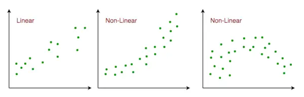
• Linjärt samband : Relationen mellan respons- och funktionsvariabler bör vara linjär. Linearitetsantagandet kan testas med hjälp av spridningsdiagram. Som visas nedan representerar 1:a siffran linjärt relaterade variabler medan variabler i 2:a och 3:e siffrorna sannolikt är icke-linjära. Så den första figuren ger bättre förutsägelser med linjär regression.

Linjärt samband i funktionsutrymmet

• Lite eller ingen multikollinearitet : Det antas att det finns liten eller ingen multikollinearitet i data. Multikollinearitet uppstår när egenskaperna (eller oberoende variabler) inte är oberoende av varandra.
• Liten eller ingen autokorrelation : Ett annat antagande är att det finns liten eller ingen autokorrelation i data. Autokorrelation uppstår när de kvarvarande felen inte är oberoende av varandra. Du kan hänvisa här för mer insikt i detta ämne.
• Inga extremvärden: Vi antar att det inte finns några extremvärden i uppgifterna. Outliers är datapunkter som är långt borta från resten av data. Outliers kan påverka resultaten av analysen.
• Homoskedasticitet : Homoscedasticitet beskriver en situation där feltermen (det vill säga bruset eller den slumpmässiga störningen i förhållandet mellan de oberoende variablerna och den beroende variabeln) är densamma över alla värden för de oberoende variablerna. Som visas nedan har figur 1 homoskedasticitet medan figur 2 har heteroskedasticitet.

Homoscedasticitet i linjär regression

När vi når slutet av den här artikeln diskuterar vi några tillämpningar av linjär regression nedan.

Typer av linjär regression

Det finns två huvudtyper av linjär regression:

• Enkel linjär regression: Detta innebär att förutsäga en beroende variabel baserad på en enda oberoende variabel.
• Multipel linjär regression: Detta innebär att förutsäga en beroende variabel baserad på flera oberoende variabler.

Enkel linjär regression

Enkel linjär regression är ett tillvägagångssätt för att förutsäga en svar använder en enda funktion . Det är en av de mest grundläggande maskininlärning modeller som en maskininlärningsentusiast får veta om. I linjär regression antar vi att de två variablerna, dvs beroende och oberoende variabler, är linjärt relaterade. Därför försöker vi hitta en linjär funktion som förutsäger svarsvärdet(y) så exakt som möjligt som en funktion av egenskapen eller den oberoende variabeln(x). Låt oss överväga en datauppsättning där vi har ett värde för svar y för varje funktion x:

För allmänt sett definierar vi:

x som funktion vektor , dvs x = [x_1, x_2, …., x_n],

och så svarsvektor , dvs y = [y_1, y_2, …., y_n]

för n observationer (i exemplet ovan, n=10). Ett spridningsdiagram för ovanstående datauppsättning ser ut så här:-

Spridningsdiagram för slumpmässigt genererade data

Nu är uppgiften att hitta en linje som passar bäst i ovanstående spridningsdiagram så att vi kan förutsäga svaret för eventuella nya funktionsvärden. (dvs ett värde på x som inte finns i en datauppsättning) Denna linje kallas a regressionslinje . Regressionslinjens ekvation representeras som:

h(x_i) = eta _0 + eta_1x_i

Här,

• h(x_i) representerar förutsagt svarsvärde för jag ^th observation.
• b_0 och b_1 är regressionskoefficienter och representerar y-avskärning och backe av regressionslinjen respektive.

För att skapa vår modell måste vi lära oss eller uppskatta värdena för regressionskoefficienterna b_0 och b_1. Och när vi väl har uppskattat dessa koefficienter kan vi använda modellen för att förutsäga svar!
I den här artikeln kommer vi att använda principen om Minst kvadrater .

Tänk nu på:

y_i = eta_0 + eta_1x_i + varepsilon_i = h(x_i) + varepsilon_i Rightarrow varepsilon_i = y_i -h(x_i)

Här är e_i en kvarvarande fel i iakttagelsen. Så vårt mål är att minimera det totala kvarvarande felet. Vi definierar kvadratfelet eller kostnadsfunktionen, J som:

J(eta_0,eta_1)= frac{1}{2n} sum_{i=1}^{n} varepsilon_i^{2}

Och vår uppgift är att hitta värdet av b ₀ och b ₁ för vilken J(b ₀ , b ₁ ) är minimum! Utan att gå in på de matematiska detaljerna presenterar vi resultatet här:

eta_1 = frac{SS_{xy}}{SS_{xx}}

eta_0 = ar{y} – eta_1ar{x}

Där SS _xy är summan av korsavvikelser av y och x:

SS_{xy} = sum_{i=1}^{n} (x_i-ar{x})(y_i-ar{y}) = sum_{i=1}^{n} y_ix_i – nar{x}ar{y}

Och SS _xx är summan av kvadratiska avvikelser av x:

SS_{xx} = sum_{i=1}^{n} (x_i-ar{x})^2 = sum_{i=1}^{n}x_i^2 – n(ar{x})^2

Python-implementering av enkel linjär regression

Vi kan använda Pytonorm språk för att lära sig koefficienten för linjära regressionsmodeller. För att plotta indata och bäst anpassade linje kommer vi att använda matplotlib bibliotek. Det är ett av de mest använda Python-biblioteken för att rita grafer. Här är exemplet på enkel linjär regression med Python.

Importera bibliotek

Python3

     Estimating Coefficients Function  This function, estimate_coef(), takes the input data x (independent variable) and y (dependent variable) and estimates the coefficients of the linear regression line using the least squares method.   Calculating Number of Observations:   n = np.size(x) determines the number of data points.  Calculating Means:   m_x = np.mean(x) and m_y = np.mean(y) compute the mean values of x and y, respectively.  Calculating Cross-Deviation and Deviation about x:   SS_xy = np.sum(y*x) - n*m_y*m_x and SS_xx = np.sum(x*x) - n*m_x*m_x calculate the sum of squared deviations between x and y and the sum of squared deviations of x about its mean, respectively.  Calculating Regression Coefficients:   b_1 = SS_xy / SS_xx and b_0 = m_y - b_1*m_x determine the slope (b_1) and intercept (b_0) of the regression line using the least squares method.  Returning Coefficients:   The function returns the estimated coefficients as a tuple (b_0, b_1). Python3         def estimate_coef(x, y):   # number of observations/points   n = np.size(x)     # mean of x and y vector   m_x = np.mean(x)   m_y = np.mean(y)     # calculating cross-deviation and deviation about x   SS_xy = np.sum(y*x) - n*m_y*m_x   SS_xx = np.sum(x*x) - n*m_x*m_x     # calculating regression coefficients   b_1 = SS_xy / SS_xx   b_0 = m_y - b_1*m_x     return (b_0, b_1)         Plotting Regression Line Function  This function, plot_regression_line(), takes the input data x (independent variable), y (dependent variable), and the estimated coefficients b to plot the regression line and the data points.   Plotting Scatter Plot:   plt.scatter(x, y, color = 'm', marker = 'o', s = 30) plots the original data points as a scatter plot with red markers.  Calculating Predicted Response Vector:   y_pred = b[0] + b[1]*x calculates the predicted values for y based on the estimated coefficients b.  Plotting Regression Line:   plt.plot(x, y_pred, color = 'g') plots the regression line using the predicted values and the independent variable x.  Adding Labels:   plt.xlabel('x') and plt.ylabel('y') label the x-axis as 'x' and the y-axis as 'y', respectively. Python3         def plot_regression_line(x, y, b):   # plotting the actual points as scatter plot   plt.scatter(x, y, color = 'm',   marker = 'o', s = 30)     # predicted response vector   y_pred = b[0] + b[1]*x     # plotting the regression line   plt.plot(x, y_pred, color = 'g')     # putting labels   plt.xlabel('x')   plt.ylabel('y')         Output:    Scatterplot of the points along with the regression line   Main Function  The provided code implements simple linear regression analysis by defining a function main() that performs the following steps:   Data Definition:   Defines the independent variable (x) and dependent variable (y) as NumPy arrays.  Coefficient Estimation:   Calls the estimate_coef() function to determine the coefficients of the linear regression line using the provided data.  Printing Coefficients:   Prints the estimated intercept (b_0) and slope (b_1) of the regression line. Python3         def main():   # observations / data   x = np.array([0, 1, 2, 3, 4, 5, 6, 7, 8, 9])   y = np.array([1, 3, 2, 5, 7, 8, 8, 9, 10, 12])     # estimating coefficients   b = estimate_coef(x, y)   print('Estimated coefficients:
b_0 = {}    
b_1 = {}'.format(b        Output:    Estimated coefficients: b_0 = -0.0586206896552 b_1 = 1.45747126437Multiple Linear RegressionMultiple linear regression attempts to model the relationship between   two or more features   and a response by fitting a linear equation to the observed data. Clearly, it is nothing but an extension of simple linear regression. Consider a dataset with   p   features(or independent variables) and one response(or dependent variable).  Also, the dataset contains   n   rows/observations.  We define: X (  feature matrix  ) = a matrix of size   n X p   where xij denotes the values of the jth feature for ith observation.  So,   and y (  response vector  ) = a vector of size   n   where y_{i} denotes the value of response for ith observation.   The   regression line   for   p   features is represented as:   where h(x_i) is   predicted response value   for ith observation and b_0, b_1, …, b_p are the   regression coefficients  . Also, we can write:   where e_i represents a   residual error   in ith observation. We can generalize our linear model a little bit more by representing feature matrix   X   as:   So now, the linear model can be expressed in terms of matrices as:   where,   and  Now, we determine an   estimate of b  , i.e. b’ using the   Least Squares method  . As already explained, the Least Squares method tends to determine b’ for which total residual error is minimized. We present the result directly here:   where ‘ represents the transpose of the matrix while -1 represents the  matrix inverse . Knowing the least square estimates, b’, the multiple linear regression model can now be estimated as:  where y’ is the   estimated response vector  .   Python Implementation of Multiple Linear Regression  For  multiple linear regression  using Python, we will use the Boston house pricing dataset.  Importing Libraries Python3         from sklearn.model_selection import train_test_split  import matplotlib.pyplot as plt  import numpy as np  from sklearn import datasets, linear_model, metrics  import pandas as pd         Loading the Boston Housing Dataset  The code downloads the Boston Housing dataset from the provided URL and reads it into a Pandas DataFrame (raw_df) Python3         data_url = ' http://lib.stat.cmu.edu/datasets/boston ' raw_df = pd.read_csv(data_url, sep='s+',   skiprows=22, header=None)        Preprocessing Data  This extracts the input variables (X) and target variable (y) from the DataFrame. The input variables are selected from every other row to match the target variable, which is available every other row. Python3         X = np.hstack([raw_df.values[::2, :],   raw_df.values[1::2, :2]])  y = raw_df.values[1::2, 2]        Splitting Data into Training and Testing Sets  Here it divides the data into training and testing sets using the train_test_split() function from scikit-learn. The test_size parameter specifies that 40% of the data should be used for testing. Python3         X_train, X_test,   y_train, y_test = train_test_split(X, y,   test_size=0.4,   random_state=1)        Creating and Training the Linear Regression Model  This initializes a LinearRegression object (reg) and trains the model using the training data (X_train, y_train) Python3         reg = linear_model.LinearRegression()  reg.fit(X_train, y_train)        Evaluating Model Performance  Evaluates the model’s performance by printing the regression coefficients and calculating the variance score, which measures the proportion of explained variance. A score of 1 indicates perfect prediction. Python3         # regression coefficients  print('Coefficients: ', reg.coef_)    # variance score: 1 means perfect prediction  print('Variance score: {}'.format(reg.score(X_test, y_test)))        Output:    Coefficients: [ -8.80740828e-02 6.72507352e-02 5.10280463e-02 2.18879172e+00 -1.72283734e+01 3.62985243e+00 2.13933641e-03 -1.36531300e+00 2.88788067e-01 -1.22618657e-02 -8.36014969e-01 9.53058061e-03 -5.05036163e-01] Variance score: 0.720898784611  Plotting Residual Errors   Plotting and analyzing the residual errors, which represent the difference between the predicted values and the actual values. Python3         # plot for residual error    # setting plot style  plt.style.use('fivethirtyeight')    # plotting residual errors in training data  plt.scatter(reg.predict(X_train),   reg.predict(X_train) - y_train,   color='green', s=10,   label='Train data')    # plotting residual errors in test data  plt.scatter(reg.predict(X_test),   reg.predict(X_test) - y_test,   color='blue', s=10,   label='Test data')    # plotting line for zero residual error  plt.hlines(y=0, xmin=0, xmax=50, linewidth=2)    # plotting legend  plt.legend(loc='upper right')    # plot title  plt.title('Residual errors')    # method call for showing the plot  plt.show()         Output:    Residual Error Plot for the Multiple Linear Regression In the above example, we determine the accuracy score using   Explained Variance Score  . We define:  explained_variance_score = 1 – Var{y – y’}/Var{y}  where y’ is the estimated target output, y is the corresponding (correct) target output, and Var is Variance, the square of the standard deviation. The best possible score is 1.0, lower values are worse. Polynomial Linear Regression  Polynomial Regression   is a form of linear regression in which the relationship between the independent variable x and dependent variable y is modeled as an   nth-degree   polynomial. Polynomial regression fits a nonlinear relationship between the value of x and the corresponding conditional mean of y, denoted E(y | x).   Choosing a Degree for Polynomial Regression  The choice of degree for polynomial regression is a trade-off between bias and variance. Bias is the tendency of a model to consistently predict the same value, regardless of the true value of the dependent variable. Variance is the tendency of a model to make different predictions for the same data point, depending on the specific training data used. A higher-degree polynomial can reduce bias but can also increase variance, leading to overfitting. Conversely, a lower-degree polynomial can reduce variance but can also increase bias. There are a number of methods for choosing a degree for polynomial regression, such as cross-validation and using information criteria such as Akaike information criterion (AIC) or Bayesian information criterion (BIC). Implementation of Polynomial Regression using Python Implementing the Polynomial regression using Python: Here we will import all the necessary libraries for data analysis and machine learning tasks and then loads the ‘Position_Salaries.csv’ dataset using Pandas. It then prepares the data for modeling by handling missing values and encoding categorical data. Finally, it splits the data into training and testing sets and standardizes the numerical features using StandardScaler. Python3         import pandas as pd  import matplotlib.pyplot as plt  import seaborn as sns  import sklearn  import warnings    from sklearn.preprocessing import LabelEncoder  from sklearn.impute import KNNImputer  from sklearn.model_selection import train_test_split  from sklearn.preprocessing import StandardScaler  from sklearn.metrics import f1_score  from sklearn.ensemble import RandomForestRegressor  from sklearn.ensemble import RandomForestRegressor  from sklearn.model_selection import cross_val_score    warnings.filterwarnings('ignore')    df = pd.read_csv('Position_Salaries.csv')    X = df.iloc[:,1:2].values  y = df.iloc[:,2].values  x        Output:   array([[ 1, 45000, 0], [ 2, 50000, 4], [ 3, 60000, 8], [ 4, 80000, 5], [ 5, 110000, 3], [ 6, 150000, 7], [ 7, 200000, 6], [ 8, 300000, 9], [ 9, 500000, 1], [ 10, 1000000, 2]], dtype=int64) The code creates a linear regression model and fits it to the provided data, establishing a linear relationship between the independent and dependent variables. Python3         from sklearn.linear_model import LinearRegression  lin_reg=LinearRegression()  lin_reg.fit(X,y)      The code performs quadratic and cubic regression by generating polynomial features from the original data and fitting linear regression models to these features. This enables modeling nonlinear relationships between the independent and dependent variables. Python3         from sklearn.preprocessing import PolynomialFeatures  poly_reg2=PolynomialFeatures(degree=2)  X_poly=poly_reg2.fit_transform(X)  lin_reg_2=LinearRegression()  lin_reg_2.fit(X_poly,y)    poly_reg3=PolynomialFeatures(degree=3)  X_poly3=poly_reg3.fit_transform(X)  lin_reg_3=LinearRegression()  lin_reg_3.fit(X_poly3,y)      The code creates a scatter plot of the data point, It effectively visualizes the linear relationship between position level and salary. Python3         plt.scatter(X,y,color='red')  plt.plot(X,lin_reg.predict(X),color='green')  plt.title('Simple Linear Regression')  plt.xlabel('Position Level')  plt.ylabel('Salary')  plt.show()        Output:    The code creates a scatter plot of the data points, overlays the predicted quadratic and cubic regression lines. It effectively visualizes the nonlinear relationship between position level and salary and compares the fits of quadratic and cubic regression models. Python3         plt.style.use('fivethirtyeight')  plt.scatter(X,y,color='red')  plt.plot(X,lin_reg_2.predict(poly_reg2.fit_transform(X)),color='green')  plt.plot(X,lin_reg_3.predict(poly_reg3.fit_transform(X)),color='yellow')  plt.title('Polynomial Linear Regression Degree 2')  plt.xlabel('Position Level')  plt.ylabel('Salary')  plt.show()        Output:    The code effectively visualizes the relationship between position level and salary using cubic regression and generates a continuous prediction line for a broader range of position levels. Python3         plt.style.use('fivethirtyeight')  X_grid=np.arange(min(X),max(X),0.1) # This will give us a vector.We will have to convert this into a matrix  X_grid=X_grid.reshape((len(X_grid),1))  plt.scatter(X,y,color='red')  plt.plot(X_grid,lin_reg_3.predict(poly_reg3.fit_transform(X_grid)),color='lightgreen')    #plt.plot(X,lin_reg_3.predict(poly_reg3.fit_transform(X)),color='green')  plt.title('Polynomial Linear Regression Degree 3')  plt.xlabel('Position Level')  plt.ylabel('Salary')  plt.show()        Output:    Applications of Linear Regression  Trend lines:   A trend line represents the variation in quantitative data with the passage of time (like GDP, oil prices, etc.). These trends usually follow a linear relationship. Hence, linear regression can be applied to predict future values. However, this method suffers from a lack of scientific validity in cases where other potential changes can affect the data.  Economics:   Linear regression is the predominant empirical tool in economics. For example, it is used to predict consumer spending, fixed investment spending, inventory investment, purchases of a country’s exports, spending on imports, the demand to hold liquid assets, labor demand, and labor supply.  Finance:   The capital price asset model uses linear regression to analyze and quantify the systematic risks of an investment.  Biology:   Linear regression is used to model causal relationships between parameters in biological systems.  Advantages   of Linear Regression  Easy to interpret:   The coefficients of a linear regression model represent the change in the dependent variable for a one-unit change in the independent variable, making it simple to comprehend the relationship between the variables.  Robust to outliers:   Linear regression is relatively robust to outliers meaning it is less affected by extreme values of the independent variable compared to other statistical methods.  Can handle both linear and nonlinear relationships:   Linear regression can be used to model both linear and nonlinear relationships between variables. This is because the independent variable can be transformed before it is used in the model.  No need for feature scaling or transformation:   Unlike some machine learning algorithms, linear regression does not require feature scaling or transformation. This can be a significant advantage, especially when dealing with large datasets.  Disadvantages   of Linear Regression  Assumes linearity:   Linear regression assumes that the relationship between the independent variable and the dependent variable is linear. This assumption may not be valid for all data sets. In cases where the relationship is nonlinear, linear regression may not be a good choice.  Sensitive to multicollinearity:   Linear regression is sensitive to multicollinearity. This occurs when there is a high correlation between the independent variables. Multicollinearity can make it difficult to interpret the coefficients of the model and can lead to overfitting.  May not be suitable for highly complex relationships:   Linear regression may not be suitable for modeling highly complex relationships between variables. For example, it may not be able to model relationships that include interactions between the independent variables.  Not suitable for classification tasks:   Linear regression is a regression algorithm and is not suitable for classification tasks, which involve predicting a categorical variable rather than a continuous variable.Frequently Asked Question(FAQs)1.   How to use linear regression to make predictions?  Once a linear regression model has been trained, it can be used to make predictions for new data points. The scikit-learn LinearRegression class provides a method called predict() that can be used to make predictions. 2.  What is linear regression?  Linear regression is a supervised machine learning algorithm used to predict a continuous numerical output. It assumes that the relationship between the independent variables (features) and the dependent variable (target) is linear, meaning that the predicted value of the target can be calculated as a linear combination of the features.   3. How to perform linear regression in Python?  There are several libraries in Python that can be used to perform linear regression, including scikit-learn, statsmodels, and NumPy. The scikit-learn library is the most popular choice for machine learning tasks, and it provides a simple and efficient implementation of linear regression. 4.   What are some applications of linear regression?  Linear regression is a versatile algorithm that can be used for a wide variety of applications, including finance, healthcare, and marketing. Some specific examples include: Predicting house pricesPredicting stock pricesDiagnosing medical conditionsPredicting customer churn5. How linear regression is implemented in sklearn?Linear regression is implemented in scikit-learn using the LinearRegression class. This class provides methods to fit a linear regression model to a training dataset and predict the target value for new data points.