np.vstack : Pour empiler des tableaux le long de l'axe vertical. np.hstack : Pour empiler des tableaux le long de l'axe horizontal. np.column_stack : Pour empiler des tableaux 1D sous forme de colonnes dans des tableaux 2D. np.concaténer : Pour empiler des tableaux le long de l'axe spécifié (l'axe est passé en argument).

   import   numpy   as   np   a   =   np  .  array  ([[  1     2  ]   [  3     4  ]])   b   =   np  .  array  ([[  5     6  ]   [  7     8  ]])   # vertical stacking   print  (  'Vertical stacking:  n  '     np  .  vstack  ((  a     b  )))   # horizontal stacking   print  (  '  n  Horizontal stacking:  n  '     np  .  hstack  ((  a     b  )))   c   =   [  5     6  ]   # stacking columns   print  (  '  n  Column stacking:  n  '     np  .  column_stack  ((  a     c  )))   # concatenation method    print  (  '  n  Concatenating to 2nd axis:  n  '     np  .  concatenate  ((  a     b  )   1  ))   

Vertical stacking: [[1 2] [3 4] [5 6] [7 8]] Horizontal stacking: [[1 2 5 6] [3 4 7 8]] Column stacking: [[1 2 5] [3 4 6]] Concatenating to 2nd axis: [[1 2 5 6] [3 4 7 8]] 

np.hsplit : Diviser le tableau le long de l’axe horizontal. np.vsplit : Diviser le tableau le long de l’axe vertical. np.array_split : Diviser le tableau le long de l'axe spécifié.

   import   numpy   as   np   a   =   np  .  array  ([[  1     3     5     7     9     11  ]   [  2     4     6     8     10     12  ]])   # horizontal splitting   print  (  'Splitting along horizontal axis into 2 parts:  n  '     np  .  hsplit  (  a     2  ))   # vertical splitting   print  (  '  n  Splitting along vertical axis into 2 parts:  n  '     np  .  vsplit  (  a     2  ))   

Splitting along horizontal axis into 2 parts: [array([[1 3 5] [2 4 6]]) array([[ 7 9 11] [ 8 10 12]])] Splitting along vertical axis into 2 parts: [array([[ 1 3 5 7 9 11]]) array([[ 2 4 6 8 10 12]])] 

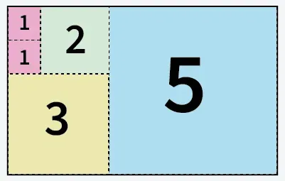
 A(2-D array): 4 x 3 B(1-D array): 3 Result : 4 x 3    
 A(4-D array): 7 x 1 x 6 x 1 B(3-D array): 3 x 1 x 5 Result : 7 x 3 x 6 x 5   But this would be a mismatch:  
 A: 4 x 3 B: 4   The simplest broadcasting example occurs when an array and a scalar value are combined in an operation. Consider the example given below: Python   
   import   numpy   as   np   a   =   np  .  array  ([  1.0     2.0     3.0  ])   # Example 1   b   =   2.0   print  (  a   *   b  )   # Example 2   c   =   [  2.0     2.0     2.0  ]   print  (  a   *   c  )   
  Output:  
[ 2. 4. 6.] [ 2. 4. 6.] 
 We can think of the scalar b being stretched during the arithmetic operation into an array with the same shape as a. The new elements in b as shown in above figure are simply copies of the original scalar. Although the stretching analogy is only conceptual. Numpy is smart enough to use the original scalar value without actually making copies so that broadcasting operations are as memory and computationally efficient as possible. Because Example 1 moves less memory (b is a scalar not an array) around during the multiplication it is about 10% faster than Example 2 using the standard numpy on Windows 2000 with one million element arrays! The figure below makes the concept more clear:    In above example the scalar b is stretched to become an array of with the same shape as a so the shapes are compatible for element-by-element multiplication. Now let us see an example where both arrays get stretched. Python   
   import   numpy   as   np   a   =   np  .  array  ([  0.0     10.0     20.0     30.0  ])   b   =   np  .  array  ([  0.0     1.0     2.0  ])   print  (  a  [:   np  .  newaxis  ]   +   b  )   
  Output:  
[[ 0. 1. 2.] [ 10. 11. 12.] [ 20. 21. 22.] [ 30. 31. 32.]]  
   Dans certains cas, la diffusion étend les deux tableaux pour former un tableau de sortie plus grand que l'un ou l'autre des tableaux initiaux.    Travailler avec datetime :   Numpy has core array data types which natively support datetime functionality. The data type is called datetime64 so named because datetime is already taken by the datetime library included in Python. Consider the example below for some examples: Python   
   import   numpy   as   np   # creating a date   today   =   np  .  datetime64  (  '2017-02-12'  )   print  (  'Date is:'     today  )   print  (  'Year is:'     np  .  datetime64  (  today     'Y'  ))   # creating array of dates in a month   dates   =   np  .  arange  (  '2017-02'     '2017-03'     dtype  =  'datetime64[D]'  )   print  (  '  n  Dates of February 2017:  n  '     dates  )   print  (  'Today is February:'     today   in   dates  )   # arithmetic operation on dates   dur   =   np  .  datetime64  (  '2017-05-22'  )   -   np  .  datetime64  (  '2016-05-22'  )   print  (  '  n  No. of days:'     dur  )   print  (  'No. of weeks:'     np  .  timedelta64  (  dur     'W'  ))   # sorting dates   a   =   np  .  array  ([  '2017-02-12'     '2016-10-13'     '2019-05-22'  ]   dtype  =  'datetime64'  )   print  (  '  n  Dates in sorted order:'     np  .  sort  (  a  ))   
  Output:  
Date is: 2017-02-12 Year is: 2017 Dates of February 2017: ['2017-02-01' '2017-02-02' '2017-02-03' '2017-02-04' '2017-02-05' '2017-02-06' '2017-02-07' '2017-02-08' '2017-02-09' '2017-02-10' '2017-02-11' '2017-02-12' '2017-02-13' '2017-02-14' '2017-02-15' '2017-02-16' '2017-02-17' '2017-02-18' '2017-02-19' '2017-02-20' '2017-02-21' '2017-02-22' '2017-02-23' '2017-02-24' '2017-02-25' '2017-02-26' '2017-02-27' '2017-02-28'] Today is February: True No. of days: 365 days No. of weeks: 52 weeks Dates in sorted order: ['2016-10-13' '2017-02-12' '2019-05-22'] 
     Algèbre linéaire dans NumPy : Le module d'algèbre linéaire de NumPy propose diverses méthodes pour appliquer l'algèbre linéaire sur n'importe quel tableau numpy. Vous pouvez trouver : 
  
trace déterminante du rang, etc. d'un tableau. 
  
propres valeurs ou matrices 
  
produits matriciels et vectoriels (produit point intérieur extérieur, etc.) exponentiation matricielle 
  
résolvez des équations linéaires ou tensorielles et bien plus encore ! 
  
 Consider the example below which explains how we can use NumPy to do some matrix operations. Python   
   import   numpy   as   np   A   =   np  .  array  ([[  6     1     1  ]   [  4     -  2     5  ]   [  2     8     7  ]])   print  (  'Rank of A:'     np  .  linalg  .  matrix_rank  (  A  ))   print  (  '  n  Trace of A:'     np  .  trace  (  A  ))   print  (  '  n  Determinant of A:'     np  .  linalg  .  det  (  A  ))   print  (  '  n  Inverse of A:  n  '     np  .  linalg  .  inv  (  A  ))   print  (  '  n  Matrix A raised to power 3:  n  '     np  .  linalg  .  matrix_power  (  A     3  ))   
  Output:  
Rank of A: 3 Trace of A: 11 Determinant of A: -306.0 Inverse of A: [[ 0.17647059 -0.00326797 -0.02287582] [ 0.05882353 -0.13071895 0.08496732] [-0.11764706 0.1503268 0.05228758]] Matrix A raised to power 3: [[336 162 228] [406 162 469] [698 702 905]] 
 Let us assume that we want to solve this linear equation set:  
 x + 2*y = 8 3*x + 4*y = 18   This problem can be solved using   linalg.solve   method as shown in example below: Python   
   import   numpy   as   np   # coefficients   a   =   np  .  array  ([[  1     2  ]   [  3     4  ]])   # constants   b   =   np  .  array  ([  8     18  ])   print  (  'Solution of linear equations:'     np  .  linalg  .  solve  (  a     b  ))   
  Output:  
Solution of linear equations: [ 2. 3.] 
 Finally we see an example which shows how one can perform linear regression using least squares method. A linear regression line is of the form w1  x + w 2 = y et c'est la ligne qui minimise la somme des carrés de la distance de chaque point de données à la ligne. Ainsi, étant donné n paires de données (xi yi), les paramètres que nous recherchons sont w1 et w2 qui minimisent l'erreur :  Let us have a look at the example below: Python   
   import   numpy   as   np   import   matplotlib.pyplot   as   plt   # x co-ordinates   x   =   np  .  arange  (  0     9  )   A   =   np  .  array  ([  x     np  .  ones  (  9  )])   # linearly generated sequence   y   =   [  19     20     20.5     21.5     22     23     23     25.5     24  ]   # obtaining the parameters of regression line   w   =   np  .  linalg  .  lstsq  (  A  .  T     y  )[  0  ]   # plotting the line   line   =   w  [  0  ]  *  x   +   w  [  1  ]   # regression line   plt  .  plot  (  x     line     'r-'  )   plt  .  plot  (  x     y     'o'  )   plt  .  show  ()   
  Output: