Python으로 DSA 배우기 | Python 데이터 구조 및 알고리즘
이 튜토리얼은 초보자에게 친숙한 가이드입니다. 데이터 구조와 알고리즘 학습 파이썬을 사용하여. 이 기사에서는 목록, 튜플, 사전 등과 같은 내장 데이터 구조와 다음과 같은 일부 사용자 정의 데이터 구조에 대해 설명합니다. 연결리스트 , 나무 , 그래프 , 등, 훌륭하고 잘 설명된 예제와 연습 문제의 도움으로 검색 및 정렬 알고리즘을 탐색할 수 있습니다.

기울기
파이썬 목록 다른 프로그래밍 언어의 배열과 마찬가지로 순서가 지정된 데이터 모음입니다. 목록에 다양한 유형의 요소가 허용됩니다. Python List의 구현은 C++의 벡터 또는 JAVA의 ArrayList와 유사합니다. 비용이 많이 드는 작업은 모든 요소를 이동해야 하기 때문에 목록의 시작 부분에서 요소를 삽입하거나 삭제하는 것입니다. 사전 할당된 메모리가 가득 차면 목록 끝에 삽입하고 삭제하는 것도 비용이 많이 들 수 있습니다.
예: Python 목록 생성
파이썬3 List = [1, 2, 3, 'GFG', 2.3] print(List)
산출
[1, 2, 3, 'GFG', 2.3]
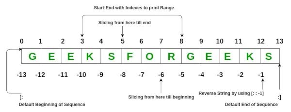
목록 요소는 할당된 인덱스로 액세스할 수 있습니다. 목록의 Python 시작 인덱스에서 시퀀스는 0이고 끝 인덱스는 (N 요소가 있는 경우) N-1입니다.
예: Python 목록 작업
파이썬3 # Creating a List with # the use of multiple values List = ['Geeks', 'For', 'Geeks'] print('
List containing multiple values: ') print(List) # Creating a Multi-Dimensional List # (By Nesting a list inside a List) List2 = [['Geeks', 'For'], ['Geeks']] print('
Multi-Dimensional List: ') print(List2) # accessing a element from the # list using index number print('Accessing element from the list') print(List[0]) print(List[2]) # accessing a element using # negative indexing print('Accessing element using negative indexing') # print the last element of list print(List[-1]) # print the third last element of list print(List[-3]) 산출
List containing multiple values: ['Geeks', 'For', 'Geeks'] Multi-Dimensional List: [['Geeks', 'For'], ['Geeks']] Accessing element from the list Geeks Geeks Accessing element using negative indexing Geeks Geeks
튜플
파이썬 튜플 리스트와 유사하지만 튜플은 불변 본질적으로 즉, 일단 생성되면 수정할 수 없습니다. 리스트와 마찬가지로 튜플에도 다양한 유형의 요소가 포함될 수 있습니다.
Python에서 튜플은 데이터 시퀀스 그룹화를 위해 괄호를 사용하거나 사용하지 않고 '쉼표'로 구분된 값 시퀀스를 배치하여 생성됩니다.
메모: 한 요소의 튜플을 만들려면 뒤에 쉼표가 있어야 합니다. 예를 들어 (8,)은 8을 요소로 포함하는 튜플을 생성합니다.
예: Python 튜플 작업
파이썬3 # Creating a Tuple with # the use of Strings Tuple = ('Geeks', 'For') print('
Tuple with the use of String: ') print(Tuple) # Creating a Tuple with # the use of list list1 = [1, 2, 4, 5, 6] print('
Tuple using List: ') Tuple = tuple(list1) # Accessing element using indexing print('First element of tuple') print(Tuple[0]) # Accessing element from last # negative indexing print('
Last element of tuple') print(Tuple[-1]) print('
Third last element of tuple') print(Tuple[-3]) 산출
Tuple with the use of String: ('Geeks', 'For') Tuple using List: First element of tuple 1 Last element of tuple 6 Third last element of tuple 4 세트
파이썬 세트 중복을 허용하지 않는 변경 가능한 데이터 모음입니다. 세트는 기본적으로 멤버십 테스트를 포함하고 중복 항목을 제거하는 데 사용됩니다. 여기에 사용된 데이터 구조는 평균 O(1)에서 삽입, 삭제 및 순회를 수행하는 인기 있는 기술인 해싱(Hashing)입니다.
동일한 인덱스 위치에 여러 값이 있는 경우 값이 해당 인덱스 위치에 추가되어 연결 목록을 형성합니다. 에서 CPython 세트는 더미 변수가 있는 사전을 사용하여 구현됩니다. 여기서 핵심은 시간 복잡도에 대해 더 큰 최적화로 설정된 멤버입니다.
구현 설정:

단일 HashTable에 대한 수많은 작업으로 설정:

예: Python 집합 작업
파이썬3 # Creating a Set with # a mixed type of values # (Having numbers and strings) Set = set([1, 2, 'Geeks', 4, 'For', 6, 'Geeks']) print('
Set with the use of Mixed Values') print(Set) # Accessing element using # for loop print('
Elements of set: ') for i in Set: print(i, end =' ') print() # Checking the element # using in keyword print('Geeks' in Set) 산출
Set with the use of Mixed Values {1, 2, 4, 6, 'For', 'Geeks'} Elements of set: 1 2 4 6 For Geeks True 냉동 세트
냉동 세트 Python에서 고정된 집합이나 적용되는 집합에 영향을 주지 않고 결과를 생성하는 메서드와 연산자만 지원하는 불변 객체입니다. 세트의 요소는 언제든지 수정될 수 있지만 고정된 세트의 요소는 생성 후에도 동일하게 유지됩니다.
예: Python Frozen 세트
파이썬3 # Same as {'a', 'b','c'} normal_set = set(['a', 'b','c']) print('Normal Set') print(normal_set) # A frozen set frozen_set = frozenset(['e', 'f', 'g']) print('
Frozen Set') print(frozen_set) # Uncommenting below line would cause error as # we are trying to add element to a frozen set # frozen_set.add('h') 산출
Normal Set {'a', 'b', 'c'} Frozen Set frozenset({'f', 'g', 'e'}) 끈
파이썬 문자열 유니코드 문자를 나타내는 변경할 수 없는 바이트 배열입니다. Python에는 문자 데이터 유형이 없습니다. 단일 문자는 단순히 길이가 1인 문자열입니다.
메모: 문자열은 변경할 수 없으므로 문자열을 수정하면 새 복사본이 생성됩니다.
예: Python 문자열 작업
파이썬3 String = 'Welcome to GeeksForGeeks' print('Creating String: ') print(String) # Printing First character print('
First character of String is: ') print(String[0]) # Printing Last character print('
Last character of String is: ') print(String[-1]) 산출
Creating String: Welcome to GeeksForGeeks First character of String is: W Last character of String is: s
사전
파이썬 사전 키:값 쌍 형식으로 데이터를 저장하는 정렬되지 않은 데이터 모음입니다. O(1)의 시간 복잡도를 갖는 다른 언어의 해시 테이블과 같습니다. Python 사전의 색인화는 키의 도움으로 수행됩니다. 이는 해시 가능한 유형, 즉 문자열, 숫자, 튜플 등과 같이 결코 변경될 수 없는 객체입니다. 중괄호({}) 또는 사전 이해를 사용하여 사전을 만들 수 있습니다.
예: Python 사전 작업
파이썬3 # Creating a Dictionary Dict = {'Name': 'Geeks', 1: [1, 2, 3, 4]} print('Creating Dictionary: ') print(Dict) # accessing a element using key print('Accessing a element using key:') print(Dict['Name']) # accessing a element using get() # method print('Accessing a element using get:') print(Dict.get(1)) # creation using Dictionary comprehension myDict = {x: x**2 for x in [1,2,3,4,5]} print(myDict) 산출
Creating Dictionary: {'Name': 'Geeks', 1: [1, 2, 3, 4]} Accessing a element using key: Geeks Accessing a element using get: [1, 2, 3, 4] {1: 1, 2: 4, 3: 9, 4: 16, 5: 25} 행렬
행렬은 각 요소의 크기가 완전히 동일한 2D 배열입니다. 행렬을 생성하기 위해 우리는 NumPy 패키지 .
예: Python NumPy 행렬 연산
파이썬3 import numpy as np a = np.array([[1,2,3,4],[4,55,1,2], [8,3,20,19],[11,2,22,21]]) m = np.reshape(a,(4, 4)) print(m) # Accessing element print('
Accessing Elements') print(a[1]) print(a[2][0]) # Adding Element m = np.append(m,[[1, 15,13,11]],0) print('
Adding Element') print(m) # Deleting Element m = np.delete(m,[1],0) print('
Deleting Element') print(m) 산출
[[ 1 2 3 4] [ 4 55 1 2] [ 8 3 20 19] [11 2 22 21]] Accessing Elements [ 4 55 1 2] 8 Adding Element [[ 1 2 3 4] [ 4 55 1 2] [ 8 3 20 19] [11 2 22 21] [ 1 15 13 11]] Deleting Element [[ 1 2 3 4] [ 8 3 20 19] [11 2 22 21] [ 1 15 13 11]]
바이테어레이
Python Bytearray는 0 <= x < 256 범위의 가변 정수 시퀀스를 제공합니다.
예: Python Bytearray 작업
파이썬3 # Creating bytearray a = bytearray((12, 8, 25, 2)) print('Creating Bytearray:') print(a) # accessing elements print('
Accessing Elements:', a[1]) # modifying elements a[1] = 3 print('
After Modifying:') print(a) # Appending elements a.append(30) print('
After Adding Elements:') print(a) 산출
Creating Bytearray: bytearray(b'x0cx08x19x02') Accessing Elements: 8 After Modifying: bytearray(b'x0cx03x19x02') After Adding Elements: bytearray(b'x0cx03x19x02x1e')
연결리스트
ㅏ 연결리스트 요소가 인접한 메모리 위치에 저장되지 않는 선형 데이터 구조입니다. 연결된 목록의 요소는 아래 이미지와 같이 포인터를 사용하여 연결됩니다.

연결리스트는 연결리스트의 첫 번째 노드를 가리키는 포인터로 표현됩니다. 첫 번째 노드를 헤드라고 합니다. 연결된 목록이 비어 있으면 헤드 값은 NULL입니다. 목록의 각 노드는 최소한 두 부분으로 구성됩니다.
- 데이터
- 다음 노드에 대한 포인터(또는 참조)
예: Python에서 연결 목록 정의
파이썬3 # Node class class Node: # Function to initialize the node object def __init__(self, data): self.data = data # Assign data self.next = None # Initialize # next as null # Linked List class class LinkedList: # Function to initialize the Linked # List object def __init__(self): self.head = None
3개의 노드로 구성된 간단한 연결리스트를 만들어 보겠습니다.
파이썬3 # A simple Python program to introduce a linked list # Node class class Node: # Function to initialise the node object def __init__(self, data): self.data = data # Assign data self.next = None # Initialize next as null # Linked List class contains a Node object class LinkedList: # Function to initialize head def __init__(self): self.head = None # Code execution starts here if __name__=='__main__': # Start with the empty list llist = LinkedList() llist.head = Node(1) second = Node(2) third = Node(3) ''' Three nodes have been created. We have references to these three blocks as head, second and third llist.head second third | | | | | | +----+------+ +----+------+ +----+------+ | 1 | None | | 2 | None | | 3 | None | +----+------+ +----+------+ +----+------+ ''' llist.head.next = second; # Link first node with second ''' Now next of first Node refers to second. So they both are linked. llist.head second third | | | | | | +----+------+ +----+------+ +----+------+ | 1 | o-------->| 2 | null | | 3 | null | +----+------+ +----+------+ +----+------+ ''' 두 번째.다음 = 세 번째 ; # 두 번째 노드를 세 번째 노드 '''와 연결합니다. 이제 두 번째 노드 다음은 세 번째 노드를 나타냅니다. 따라서 세 노드가 모두 연결됩니다. lllist.head 두 번째 세 번째 | | | | | | +----+------+ +----+------+ +----+------+ | 1 | 아 -------->| 2 | 아 -------->| 3 | null | +----+------+ +----+------+ +----+------+ '''
연결리스트 순회
이전 프로그램에서는 세 개의 노드로 구성된 간단한 연결 목록을 만들었습니다. 생성된 목록을 순회하여 각 노드의 데이터를 인쇄해 보겠습니다. 순회를 위해 주어진 목록을 인쇄하는 범용 함수 printList()를 작성해 보겠습니다.
파이썬3 # A simple Python program for traversal of a linked list # Node class class Node: # Function to initialise the node object def __init__(self, data): self.data = data # Assign data self.next = None # Initialize next as null # Linked List class contains a Node object class LinkedList: # Function to initialize head def __init__(self): self.head = None # This function prints contents of linked list # starting from head def printList(self): temp = self.head while (temp): print (temp.data) temp = temp.next # Code execution starts here if __name__=='__main__': # Start with the empty list llist = LinkedList() llist.head = Node(1) second = Node(2) third = Node(3) llist.head.next = second; # Link first node with second second.next = third; # Link second node with the third node llist.printList()
산출
1 2 3
연결 목록에 대한 추가 기사
- 연결리스트 삽입
- 연결 목록 삭제(주어진 키 삭제)
- 연결리스트 삭제(주어진 위치의 키 삭제)
- 연결 목록의 길이 찾기(반복 및 재귀)
- 연결 목록에서 요소 검색(반복 및 재귀)
- Linked List의 끝에서 N번째 노드
- 연결리스트 뒤집기

스택과 관련된 기능은 다음과 같습니다.
- 비어 있는() - 스택이 비어 있는지 여부를 반환 – 시간 복잡도: O(1)
- 크기() – 스택의 크기를 반환합니다. – 시간 복잡도: O(1)
- 맨 위() - 스택의 최상위 요소에 대한 참조를 반환합니다. – 시간 복잡도: O(1)
- 푸시(a) - 스택의 맨 위에 요소 'a'를 삽입합니다. – 시간 복잡도: O(1)
- 팝() - 스택의 최상위 요소를 삭제합니다. – 시간 복잡도: O(1)
  stack = [] # append() function to push # element in the stack stack.append('g') stack.append('f') stack.append('g') print('Initial stack') print(stack) # pop() function to pop # element from stack in # LIFO order print('
Elements popped from stack:') print(stack.pop()) print(stack.pop()) print(stack.pop()) print('
Stack after elements are popped:') print(stack) # uncommenting print(stack.pop()) # will cause an IndexError # as the stack is now empty
산출
Initial stack ['g', 'f', 'g'] Elements popped from stack: g f g Stack after elements are popped: []
스택에 대한 추가 기사
- 스택을 사용하여 중위에서 후위로 변환
- 접두사에서 중위사로의 변환
- 접두사에서 후위로의 변환
- 접두사에서 접두사로의 변환
- 접미사에서 중위사로
- 표현식에서 균형 잡힌 괄호를 확인하세요.
- 후위 표현의 평가
스택으로서, 대기줄 FIFO(선입선출) 방식으로 항목을 저장하는 선형 데이터 구조입니다. 대기열을 사용하면 가장 최근에 추가된 항목이 먼저 제거됩니다. 대기열의 좋은 예는 먼저 온 소비자가 먼저 제공되는 리소스에 대한 소비자 대기열입니다.

대기열과 관련된 작업은 다음과 같습니다.
- 대기열에 추가: 대기열에 항목을 추가합니다. 대기열이 가득 차면 오버플로 상태라고 합니다. – 시간 복잡도: O(1)
- 따라서: 대기열에서 항목을 제거합니다. 항목은 푸시된 순서와 동일한 순서로 팝됩니다. 큐가 비어 있으면 언더플로우 상태라고 합니다. – 시간 복잡도: O(1)
- 앞쪽: 대기열에서 맨 앞의 항목 가져오기 – 시간 복잡도: O(1)
- 뒤쪽: 대기열에서 마지막 항목 가져오기 – 시간 복잡도: O(1)
  # Initializing a queue queue = [] # Adding elements to the queue queue.append('g') queue.append('f') queue.append('g') print('Initial queue') print(queue) # Removing elements from the queue print('
Elements dequeued from queue') print(queue.pop(0)) print(queue.pop(0)) print(queue.pop(0)) print('
Queue after removing elements') print(queue) # Uncommenting print(queue.pop(0)) # will raise and IndexError # as the queue is now empty
산출
Initial queue ['g', 'f', 'g'] Elements dequeued from queue g f g Queue after removing elements []
대기열에 대한 추가 기사
- 스택을 사용하여 대기열 구현
- 대기열을 사용하여 스택 구현
- 단일 큐를 사용하여 스택 구현
우선순위 대기열
우선순위 대기열 큐의 각 데이터/값이 특정 우선순위를 갖는 추상 데이터 구조입니다. 예를 들어 항공사에서는 비즈니스 또는 일등석이라는 제목의 수하물이 나머지 수하물보다 먼저 도착합니다. 우선순위 대기열은 다음 속성을 가진 대기열의 확장입니다.
- 우선순위가 높은 요소는 우선순위가 낮은 요소보다 먼저 대기열에서 제거됩니다.
- 두 요소의 우선순위가 동일한 경우 대기열의 순서에 따라 서비스됩니다.
# A simple implementation of Priority Queue # using Queue. class PriorityQueue(object): def __init__(self): self.queue = [] def __str__(self): return ' '.join([str(i) for i in self.queue]) # for checking if the queue is empty def isEmpty(self): return len(self.queue) == 0 # for inserting an element in the queue def insert(self, data): self.queue.append(data) # for popping an element based on Priority def delete(self): try: max = 0 for i in range(len(self.queue)): if self.queue[i]>self.queue[max]: max = i item = self.queue[max] del self.queue[max] IndexError: print()exit() if __name__ == '__main__': myQueue = PriorityQueue(를 제외한 항목 반환 ) myQueue.insert(12) myQueue.insert(1) myQueue.insert(14) myQueue.insert(7) print(myQueue) myQueue.isEmpty()가 아닌 경우: print(myQueue.delete())
산출
12 1 14 7 14 12 7 1
더미
Python의 heapq 모듈 우선순위 큐를 표현하는데 주로 사용되는 힙 데이터 구조를 제공합니다. 이 데이터 구조의 속성은 요소가 팝될 때마다 항상 가장 작은 요소(최소 힙)를 제공한다는 것입니다. 요소가 푸시되거나 팝될 때마다 힙 구조가 유지됩니다. heap[0] 요소는 매번 가장 작은 요소도 반환합니다. O(log n) 시간에 가장 작은 요소의 추출 및 삽입을 지원합니다.
일반적으로 힙은 두 가지 유형이 있습니다.
- 최대 힙: Max-Heap에서 루트 노드에 있는 키는 모든 하위 노드에 있는 키 중에서 가장 커야 합니다. 해당 이진 트리의 모든 하위 트리에 대해 동일한 속성이 반복적으로 true여야 합니다.
- 최소 힙: 최소 힙에서 루트 노드에 있는 키는 모든 하위 노드에 있는 키 중에서 최소값이어야 합니다. 해당 이진 트리의 모든 하위 트리에 대해 동일한 속성이 반복적으로 true여야 합니다.

# importing 'heapq' to implement heap queue import heapq # initializing list li = [5, 7, 9, 1, 3] # using heapify to convert list into heap heapq.heapify(li) # printing created heap print ('The created heap is : ',end='') print (list(li)) # using heappush() to push elements into heap # pushes 4 heapq.heappush(li,4) # printing modified heap print ('The modified heap after push is : ',end='') print (list(li)) # using heappop() to pop smallest element print ('The popped and smallest element is : ',end='') print (heapq.heappop(li)) 산출
The created heap is : [1, 3, 9, 7, 5] The modified heap after push is : [1, 3, 4, 7, 5, 9] The popped and smallest element is : 1
힙에 대한 추가 기사
- 바이너리 힙
- 배열에서 K번째로 큰 요소
- 정렬되지 않은 배열에서 K번째 최소/최대 요소
- 거의 정렬된 배열 정렬
- K번째로 큰 합계 연속 하위 배열
- 배열의 숫자로 구성된 두 숫자의 최소 합
트리는 아래 그림과 같은 계층적 데이터 구조입니다.
tree ---- j <-- root / f k / a h z <-- leaves
트리의 최상위 노드를 루트(root)라고 하고, 최하위 노드나 자식이 없는 노드를 리프 노드(leaf node)라고 합니다. 노드 바로 아래에 있는 노드를 하위 노드라고 하고, 노드 바로 위에 있는 노드를 상위 노드라고 합니다.
ㅏ 이진 트리 요소가 거의 두 명의 자식을 가질 수 있는 트리입니다. 이진 트리의 각 요소에는 자식이 2개만 있을 수 있으므로 일반적으로 왼쪽 및 오른쪽 자식으로 이름을 지정합니다. 이진 트리 노드에는 다음 부분이 포함됩니다.
- 데이터
- 왼쪽 자식에 대한 포인터
- 올바른 자식에 대한 포인터
예: 노드 클래스 정의
파이썬3 # A Python class that represents an individual node # in a Binary Tree class Node: def __init__(self,key): self.left = None self.right = None self.val = key
이제 Python에서 4개의 노드가 있는 트리를 만들어 보겠습니다. 트리 구조가 아래와 같다고 가정해 보겠습니다.
tree ---- 1 <-- root / 2 3 / 4
예: 트리에 데이터 추가
파이썬3 # Python program to introduce Binary Tree # A class that represents an individual node in a # Binary Tree class Node: def __init__(self,key): self.left = None self.right = None self.val = key # create root root = Node(1) ''' following is the tree after above statement 1 / None None''' root.left = Node(2); root.right = Node(3); ''' 2 and 3 become left and right children of 1 1 / 2 3 / / None None None None''' root.left.left = Node(4); '''4 becomes left child of 2 1 / 2 3 / / 4 None None None / None None'''
트리 순회
나무를 횡단할 수 있다 다른 방법으로. 다음은 트리를 횡단하는 데 일반적으로 사용되는 방법입니다. 아래 트리를 고려해 보겠습니다.
tree ---- 1 <-- root / 2 3 / 4 5
깊이 우선 순회:
- 중위(왼쪽, 루트, 오른쪽) : 4 2 5 1 3
- 예약주문(루트, 왼쪽, 오른쪽) : 1 2 4 5 3
- 후위(왼쪽, 오른쪽, 루트) : 4 5 2 3 1
알고리즘 순서(트리)
- 왼쪽 하위 트리를 탐색합니다. 즉, Inorder(left-subtree)를 호출합니다.
- 루트를 방문하십시오.
- 오른쪽 하위 트리를 탐색합니다. 즉, Inorder(right-subtree)를 호출합니다.
알고리즘 선주문(트리)
- 루트를 방문하십시오.
- 왼쪽 하위 트리를 탐색합니다. 즉, Preorder(left-subtree)를 호출합니다.
- 오른쪽 하위 트리를 탐색합니다. 즉, Preorder(right-subtree)를 호출합니다.
알고리즘 우편순서(트리)
- 왼쪽 하위 트리를 탐색합니다. 즉, Postorder(left-subtree)를 호출합니다.
- 오른쪽 하위 트리를 탐색합니다. 즉, Postorder(right-subtree)를 호출합니다.
- 루트를 방문하십시오.
  # Python program to for tree traversals # A class that represents an individual node in a # Binary Tree class Node: def __init__(self, key): self.left = None self.right = None self.val = key # A function to do inorder tree traversal def printInorder(root): if root: # First recur on left child printInorder(root.left) # then print the data of node print(root.val), # now recur on right child printInorder(root.right) # A function to do postorder tree traversal def printPostorder(root): if root: # First recur on left child printPostorder(root.left) # the recur on right child printPostorder(root.right) # now print the data of node print(root.val), # A function to do preorder tree traversal def printPreorder(root): if root: # First print the data of node print(root.val), # Then recur on left child printPreorder(root.left) # Finally recur on right child printPreorder(root.right) # Driver code root = Node(1) root.left = Node(2) root.right = Node(3) root.left.left = Node(4) root.left.right = Node(5) print('Preorder traversal of binary tree is') printPreorder(root) print('
Inorder traversal of binary tree is') printInorder(root) print('
Postorder traversal of binary tree is') printPostorder(root)
산출
Preorder traversal of binary tree is 1 2 4 5 3 Inorder traversal of binary tree is 4 2 5 1 3 Postorder traversal of binary tree is 4 5 2 3 1
시간 복잡도 - O(n)
너비 우선 또는 레벨 순서 순회
레벨 순서 순회 트리의 너비 우선 순회는 트리에 대한 너비 우선 순회입니다. 위 트리의 레벨 순서 순회는 1 2 3 4 5입니다.
각 노드에 대해 먼저 노드를 방문한 다음 해당 하위 노드를 FIFO 대기열에 넣습니다. 아래는 동일한 알고리즘입니다.
- 빈 대기열 만들기 q
- temp_node = 루트 /*루트에서 시작*/
- temp_node가 NULL이 아닌 동안 루프
- temp_node->data를 인쇄합니다.
- temp_node의 자식(먼저 왼쪽, 오른쪽 자식)을 q에 대기열에 넣습니다.
- q에서 노드 대기열 제거
# Python program to print level # order traversal using Queue # A node structure class Node: # A utility function to create a new node def __init__(self ,key): self.data = key self.left = None self.right = None # Iterative Method to print the # height of a binary tree def printLevelOrder(root): # Base Case if root is None: return # Create an empty queue # for level order traversal queue = [] # Enqueue Root and initialize height queue.append(root) while(len(queue)>0): # 대기열의 앞 부분을 인쇄하고 # 대기열에서 제거합니다. print (queue[0].data) node = queue.pop(0) # node.left가 None이 아닌 경우 왼쪽 자식을 대기열에 넣습니다: queue.append(node.left ) # node.right가 None이 아닌 경우 오른쪽 자식을 큐에 넣습니다. queue.append(node.right) # 위 함수를 테스트하기 위한 드라이버 프로그램 root = Node(1) root.left = Node(2) root.right = Node(3) root.left.left = Node(4) root.left.right = Node(5) print ('이진 트리의 레벨 순서 탐색은 -') printLevelOrder(root) 산출
Level Order Traversal of binary tree is - 1 2 3 4 5
시간 복잡도: O(n)
이진 트리에 대한 추가 기사
- 이진 트리에 삽입
- 이진 트리에서의 삭제
- 재귀 없는 중위 트리 순회
- 재귀와 스택이 없는 중위 트리 순회!
- 주어진 Inorder 및 Preorder 순회에서 Postorder 순회를 인쇄합니다.
- 선주문 순회에서 BST의 후순 순회를 찾습니다.
이진 검색 트리 다음과 같은 속성을 갖는 노드 기반 이진 트리 데이터 구조입니다.
- 노드의 왼쪽 하위 트리에는 해당 노드의 키보다 작은 키를 가진 노드만 포함됩니다.
- 노드의 오른쪽 하위 트리에는 해당 노드의 키보다 큰 키를 가진 노드만 포함됩니다.
- 왼쪽 및 오른쪽 하위 트리도 각각 이진 검색 트리여야 합니다.

위의 이진 검색 트리 속성은 검색, 최소 및 최대와 같은 작업을 빠르게 수행할 수 있도록 키 간의 순서를 제공합니다. 순서가 없으면 주어진 키를 검색하기 위해 모든 키를 비교해야 할 수도 있습니다.
요소 검색
- 루트부터 시작하세요.
- 검색 요소를 루트와 비교하여 루트보다 작으면 왼쪽으로 반복하고, 그렇지 않으면 오른쪽으로 반복합니다.
- 검색할 요소가 어디에서나 발견되면 true를 반환하고, 그렇지 않으면 false를 반환합니다.
# A utility function to search a given key in BST def search(root,key): # Base Cases: root is null or key is present at root if root is None or root.val == key: return root # Key is greater than root's key if root.val < key: return search(root.right,key) # Key is smaller than root's key return search(root.left,key)
키 삽입
- 루트부터 시작하세요.
- 삽입 요소를 루트와 비교하여 루트보다 작으면 왼쪽으로 반복하고 그렇지 않으면 오른쪽으로 반복합니다.
- 끝에 도달한 후 해당 노드를 왼쪽에 삽입하고(현재보다 작은 경우) 오른쪽에 삽입합니다.
# Python program to demonstrate # insert operation in binary search tree # A utility class that represents # an individual node in a BST class Node: def __init__(self, key): self.left = None self.right = None self.val = key # A utility function to insert # a new node with the given key def insert(root, key): if root is None: return Node(key) else: if root.val == key: return root elif root.val < key: root.right = insert(root.right, key) else: root.left = insert(root.left, key) return root # A utility function to do inorder tree traversal def inorder(root): if root: inorder(root.left) print(root.val) inorder(root.right) # Driver program to test the above functions # Let us create the following BST # 50 # / # 30 70 # / / # 20 40 60 80 r = Node(50) r = insert(r, 30) r = insert(r, 20) r = insert(r, 40) r = insert(r, 70) r = insert(r, 60) r = insert(r, 80) # Print inorder traversal of the BST inorder(r)
산출
20 30 40 50 60 70 80
이진 검색 트리에 대한 추가 기사
- 이진 검색 트리 – 삭제 키
- 주어진 선주문 순회에서 BST 구성 | 세트 1
- 이진 트리에서 이진 검색 트리로의 변환
- 이진 검색 트리에서 최소값을 갖는 노드 찾기
- 이진 트리가 BST인지 확인하는 프로그램
ㅏ 그래프 노드와 에지로 구성된 비선형 데이터 구조입니다. 노드는 정점이라고도 하며 가장자리는 그래프의 두 노드를 연결하는 선 또는 호입니다. 보다 공식적으로 그래프는 유한한 정점(또는 노드) 집합과 노드 쌍을 연결하는 가장자리 집합으로 구성된 그래프로 정의할 수 있습니다.

위 그래프에서 정점 집합 V = {0,1,2,3,4}이고 간선 집합 E = {01, 12, 23, 34, 04, 14, 13}입니다. 다음 두 가지는 가장 일반적으로 사용되는 그래프 표현입니다.
- 인접 행렬
- 인접 목록
인접 행렬
인접 행렬(Adjacency Matrix)은 V x V 크기의 2D 배열입니다. 여기서 V는 그래프의 정점 수입니다. 2D 배열을 adj[][]라고 가정하면, 슬롯 adj[i][j] = 1은 정점 i에서 정점 j까지의 가장자리가 있음을 나타냅니다. 무방향 그래프의 인접 행렬은 항상 대칭입니다. 인접 행렬은 가중치 그래프를 나타내는 데에도 사용됩니다. adj[i][j] = w이면 정점 i에서 정점 j까지 가중치가 w인 간선이 있습니다.
파이썬3 # A simple representation of graph using Adjacency Matrix class Graph: def __init__(self,numvertex): self.adjMatrix = [[-1]*numvertex for x in range(numvertex)] self.numvertex = numvertex self.vertices = {} self.verticeslist =[0]*numvertex def set_vertex(self,vtx,id): if 0 <=vtx <=self.numvertex: self.vertices[id] = vtx self.verticeslist[vtx] = id def set_edge(self,frm,to,cost=0): frm = self.vertices[frm] to = self.vertices[to] self.adjMatrix[frm][to] = cost # for directed graph do not add this self.adjMatrix[to][frm] = cost def get_vertex(self): return self.verticeslist def get_edges(self): edges=[] for i in range (self.numvertex): for j in range (self.numvertex): if (self.adjMatrix[i][j]!=-1): edges.append((self.verticeslist[i],self.verticeslist[j],self.adjMatrix[i][j])) return edges def get_matrix(self): return self.adjMatrix G =Graph(6) G.set_vertex(0,'a') G.set_vertex(1,'b') G.set_vertex(2,'c') G.set_vertex(3,'d') G.set_vertex(4,'e') G.set_vertex(5,'f') G.set_edge('a','e',10) G.set_edge('a','c',20) G.set_edge('c','b',30) G.set_edge('b','e',40) G.set_edge('e','d',50) G.set_edge('f','e',60) print('Vertices of Graph') print(G.get_vertex()) print('Edges of Graph') print(G.get_edges()) print('Adjacency Matrix of Graph') print(G.get_matrix()) 산출
그래프의 정점
['a', 'b', 'c', 'd', 'e', 'f']
그래프의 가장자리
[('a', 'c', 20), ('a', 'e', 10), ('b', 'c', 30), ('b', 'e', 40), ( 'c', 'a', 20), ('c', 'b', 30), ('d', 'e', 50), ('e', 'a', 10), ('e ', 'b', 40), ('e', 'd', 50), ('e', 'f', 60), ('f', 'e', 60)]
그래프의 인접 행렬
[[-1, -1, 20, -1, 10, -1], [-1, -1, 30, -1, 40, -1], [20, 30, -1, -1, -1 , -1], [-1, -1, -1, -1, 50, -1], [10, 40, -1, 50, -1, 60], [-1, -1, -1, -1, 60, -1]]
인접 목록
목록의 배열이 사용됩니다. 배열의 크기는 정점의 수와 같습니다. 배열을 array[]로 둡니다. 항목 array[i]는 i번째 꼭지점에 인접한 꼭지점의 목록을 나타냅니다. 이 표현은 가중치 그래프를 나타내는 데에도 사용할 수 있습니다. 간선의 가중치는 쌍 목록으로 표현될 수 있습니다. 다음은 위 그래프의 인접 목록 표현입니다.

  # A class to represent the adjacency list of the node class AdjNode: def __init__(self, data): self.vertex = data self.next = None # A class to represent a graph. A graph # is the list of the adjacency lists. # Size of the array will be the no. of the # vertices 'V' class Graph: def __init__(self, vertices): self.V = vertices self.graph = [None] * self.V # Function to add an edge in an undirected graph def add_edge(self, src, dest): # Adding the node to the source node node = AdjNode(dest) node.next = self.graph[src] self.graph[src] = node # Adding the source node to the destination as # it is the undirected graph node = AdjNode(src) node.next = self.graph[dest] self.graph[dest] = node # Function to print the graph def print_graph(self): for i in range(self.V): print('Adjacency list of vertex {}
 head'.format(i), end='') temp = self.graph[i] while temp: print(' ->{}'.format(temp.vertex), end='') temp = temp.next print('
') # 위 그래프 클래스에 대한 드라이버 프로그램 if __name__ == '__main__' : V = 5 그래프 = Graph(V) graph.add_edge(0, 1) graph.add_edge(0, 4) graph.add_edge(1, 2) graph.add_edge(1, 3) graph.add_edge(1, 4) graph.add_edge(2, 3) graph.add_edge(3, 4) graph.print_graph()
산출
Adjacency list of vertex 0 head ->4 -> 1 정점 1 머리의 인접 목록 -> 4 -> 3 -> 2 -> 0 정점 2 머리의 인접 목록 -> 3 -> 1 정점 3 머리의 인접 목록 -> 4 -> 2 -> 1 인접 목록 정점 4 머리 목록 -> 3 -> 1 -> 0
그래프 순회
너비 우선 검색(BFS)
너비 우선 순회 그래프의 경우 트리의 너비 우선 순회와 유사합니다. 여기서 유일한 문제는 트리와 달리 그래프에 사이클이 포함될 수 있으므로 동일한 노드에 다시 올 수 있다는 것입니다. 노드를 두 번 이상 처리하지 않으려면 부울 방문 배열을 사용합니다. 단순화를 위해 시작 정점에서 모든 정점에 도달할 수 있다고 가정합니다.
예를 들어, 다음 그래프에서는 정점 2에서 순회를 시작합니다. 정점 0에 도달하면 인접한 모든 정점을 찾습니다. 2도 0의 인접한 정점입니다. 방문한 정점을 표시하지 않으면 2가 다시 처리되어 비종료 프로세스가 됩니다. 다음 그래프의 너비 우선 순회는 2, 0, 3, 1입니다.

# Python3 Program to print BFS traversal # from a given source vertex. BFS(int s) # traverses vertices reachable from s. from collections import defaultdict # This class represents a directed graph # using adjacency list representation class Graph: # Constructor def __init__(self): # default dictionary to store graph self.graph = defaultdict(list) # function to add an edge to graph def addEdge(self,u,v): self.graph[u].append(v) # Function to print a BFS of graph def BFS(self, s): # Mark all the vertices as not visited visited = [False] * (max(self.graph) + 1) # Create a queue for BFS queue = [] # Mark the source node as # visited and enqueue it queue.append(s) visited[s] = True while queue: # Dequeue a vertex from # queue and print it s = queue.pop(0) print (s, end = ' ') # Get all adjacent vertices of the # dequeued vertex s. If a adjacent # has not been visited, then mark it # visited and enqueue it for i in self.graph[s]: if visited[i] == False: queue.append(i) visited[i] = True # Driver code # Create a graph given in # the above diagram g = Graph() g.addEdge(0, 1) g.addEdge(0, 2) g.addEdge(1, 2) g.addEdge(2, 0) g.addEdge(2, 3) g.addEdge(3, 3) print ('Following is Breadth First Traversal' ' (starting from vertex 2)') g.BFS(2) 산출
Following is Breadth First Traversal (starting from vertex 2) 2 0 3 1
시간 복잡도: O(V+E) 여기서 V는 그래프의 정점 수이고 E는 그래프의 가장자리 수입니다.
깊이 우선 검색 또는 DFS
깊이 우선 순회 그래프의 경우 트리의 깊이 우선 순회와 유사합니다. 여기서 유일한 문제는 트리와 달리 그래프에 주기가 포함될 수 있고 노드를 두 번 방문할 수 있다는 것입니다. 노드를 두 번 이상 처리하지 않으려면 부울 방문 배열을 사용하십시오.
연산:
- 노드의 인덱스와 방문한 배열을 사용하는 재귀 함수를 만듭니다.
- 현재 노드를 방문한 것으로 표시하고 노드를 인쇄합니다.
- 인접 노드와 표시되지 않은 노드를 모두 순회하고 인접 노드의 인덱스를 사용하여 재귀 함수를 호출합니다.
# Python3 program to print DFS traversal # from a given graph from collections import defaultdict # This class represents a directed graph using # adjacency list representation class Graph: # Constructor def __init__(self): # default dictionary to store graph self.graph = defaultdict(list) # function to add an edge to graph def addEdge(self, u, v): self.graph[u].append(v) # A function used by DFS def DFSUtil(self, v, visited): # Mark the current node as visited # and print it visited.add(v) print(v, end=' ') # Recur for all the vertices # adjacent to this vertex for neighbour in self.graph[v]: if neighbour not in visited: self.DFSUtil(neighbour, visited) # The function to do DFS traversal. It uses # recursive DFSUtil() def DFS(self, v): # Create a set to store visited vertices visited = set() # Call the recursive helper function # to print DFS traversal self.DFSUtil(v, visited) # Driver code # Create a graph given # in the above diagram g = Graph() g.addEdge(0, 1) g.addEdge(0, 2) g.addEdge(1, 2) g.addEdge(2, 0) g.addEdge(2, 3) g.addEdge(3, 3) print('Following is DFS from (starting from vertex 2)') g.DFS(2) 산출
Following is DFS from (starting from vertex 2) 2 0 1 3
그래프에 대한 추가 기사
- 세트와 해시를 사용한 그래프 표현
- 그래프에서 Mother Vertex 찾기
- 반복 깊이 우선 검색
- BFS를 사용하여 트리의 특정 수준에 있는 노드 수 계산
- 두 정점 사이의 가능한 모든 경로 수 계산
함수가 자신을 직접 또는 간접적으로 호출하는 과정을 재귀라고 하며 해당 함수를 호출합니다. 재귀 함수 . 재귀 알고리즘을 사용하면 특정 문제를 매우 쉽게 해결할 수 있습니다. 이러한 문제의 예로는 Towers of Hanoi(TOH), Inorder/Preorder/Postorder Tree Traversals, DFS of Graph 등이 있습니다.
재귀의 기본 조건은 무엇입니까?
재귀 프로그램에서는 기본 사례에 대한 솔루션이 제공되고 더 큰 문제의 솔루션은 더 작은 문제의 관점에서 표현됩니다.
def fact(n): # base case if (n <= 1) return 1 else return n*fact(n-1)
위의 예에서는 n <= 1에 대한 기본 사례가 정의되어 있으며 기본 사례에 도달할 때까지 더 작은 값으로 변환하여 더 큰 숫자 값을 해결할 수 있습니다.
재귀에서 다른 함수 호출에 메모리가 어떻게 할당됩니까?
main()에서 함수가 호출되면 메모리가 스택에 할당됩니다. 재귀 함수는 자신을 호출하고, 호출된 함수에 대한 메모리는 호출 함수에 할당된 메모리 위에 할당되며, 각 함수 호출에 대해 다른 지역 변수 복사본이 생성됩니다. 기본 사례에 도달하면 함수는 해당 값을 호출한 함수에 반환하고 메모리 할당이 취소되고 프로세스가 계속됩니다.
간단한 함수를 사용하여 재귀가 어떻게 작동하는지 예를 들어 보겠습니다.
파이썬3 # A Python 3 program to # demonstrate working of # recursion def printFun(test): if (test < 1): return else: print(test, end=' ') printFun(test-1) # statement 2 print(test, end=' ') return # Driver Code test = 3 printFun(test)
산출
3 2 1 1 2 3
메모리 스택은 아래 다이어그램에 표시되어 있습니다.
재귀에 대한 추가 기사
- 재귀
- Python의 재귀
- 재귀 연습 문제 | 세트 1
- 재귀 연습 문제 | 세트 2
- 재귀 연습 문제 | 세트 3
- 재귀 연습 문제 | 세트 4
- 재귀 연습 문제 | 세트 5
- 재귀 연습 문제 | 세트 6
- 재귀 연습 문제 | 세트 7
>>> 더 보기
동적 프로그래밍
동적 프로그래밍 주로 일반 재귀에 대한 최적화입니다. 동일한 입력을 반복적으로 호출하는 재귀 솔루션을 볼 때마다 동적 프로그래밍을 사용하여 이를 최적화할 수 있습니다. 아이디어는 하위 문제의 결과를 간단히 저장하여 나중에 필요할 때 다시 계산할 필요가 없도록 하는 것입니다. 이 간단한 최적화는 시간 복잡성을 지수에서 다항식으로 줄여줍니다. 예를 들어 피보나치 수에 대한 간단한 재귀 솔루션을 작성하면 기하급수적인 시간 복잡도가 발생하고 하위 문제의 솔루션을 저장하여 최적화하면 시간 복잡성이 선형으로 감소합니다.

표 작성과 메모
하위 문제의 값을 재사용할 수 있도록 값을 저장하는 방법에는 두 가지가 있습니다. 여기에서는 동적 프로그래밍(DP) 문제를 해결하는 두 가지 패턴에 대해 설명합니다.
- 표: 상향식
- 메모: 위에서 아래로
표
이름 그대로 밑바닥부터 시작해서 위로 쌓이는 답을 뜻합니다. 상태 전환 측면에서 논의해 보겠습니다.
DP 문제의 상태를 기본 상태로 dp[0], 대상 상태로 dp[n]을 갖는 dp[x]로 설명하겠습니다. 따라서 우리는 목적지 상태, 즉 dp[n]의 값을 찾아야 합니다.
기본 상태, 즉 dp[0]에서 전환을 시작하고 상태 전환 관계를 따라 대상 상태 dp[n]에 도달하는 경우 전환을 시작했다는 것이 매우 분명하므로 이를 상향식 접근 방식이라고 부릅니다. 하단 기본 상태를 거쳐 원하는 최상위 상태에 도달했습니다.
자, 왜 이것을 도표화 방법이라고 부르나요?
이를 알기 위해 먼저 상향식 접근 방식을 사용하여 숫자의 계승을 계산하는 코드를 작성해 보겠습니다. 다시 한 번 DP를 해결하기 위한 일반적인 절차로 먼저 상태를 정의합니다. 이 경우 상태를 dp[x]로 정의합니다. 여기서 dp[x]는 x의 계승을 찾는 것입니다.
이제 dp[x+1] = dp[x] * (x+1) 이 분명해졌습니다.
# Tabulated version to find factorial x. dp = [0]*MAXN # base case dp[0] = 1; for i in range(n+1): dp[i] = dp[i-1] * i
메모
다시 한 번 상태 전환 측면에서 설명하겠습니다. dp[n]과 같은 일부 상태에 대한 값을 찾아야 하는 경우 기본 상태, 즉 dp[0]에서 시작하는 대신 상태 전환 후 대상 상태 dp[n]에 도달할 수 있는 상태에서 답을 묻습니다. 관계라면 DP의 하향식 패션입니다.
여기서는 최상위 대상 상태에서 여정을 시작하고 최하위 기본 상태에 도달할 때까지 대상 상태에 도달할 수 있는 상태 값을 계산하여 답을 계산합니다.
다시 한 번 하향식으로 계승 문제에 대한 코드를 작성해 보겠습니다.
# Memoized version to find factorial x. # To speed up we store the values # of calculated states # initialized to -1 dp[0]*MAXN # return fact x! def solve(x): if (x==0) return 1 if (dp[x]!=-1) return dp[x] return (dp[x] = x * solve(x-1))

동적 프로그래밍에 대한 추가 기사
- 최적의 하부 구조 특성
- 겹치는 하위 문제 속성
- 피보나치 수열
- 합이 m으로 나누어지는 부분 집합
- 최대 합 증가 하위 수열
- 가장 긴 공통 부분 문자열
알고리즘 검색
선형 검색
- arr[]의 가장 왼쪽 요소부터 시작하여 x를 arr[]의 각 요소와 하나씩 비교합니다.
- x가 요소와 일치하면 인덱스를 반환합니다.
- x가 어떤 요소와도 일치하지 않으면 -1을 반환합니다.

# Python3 code to linearly search x in arr[]. # If x is present then return its location, # otherwise return -1 def search(arr, n, x): for i in range(0, n): if (arr[i] == x): return i return -1 # Driver Code arr = [2, 3, 4, 10, 40] x = 10 n = len(arr) # Function call result = search(arr, n, x) if(result == -1): print('Element is not present in array') else: print('Element is present at index', result) 산출
Element is present at index 3
위 알고리즘의 시간복잡도는 O(n)이다.
자세한 내용은 다음을 참조하세요. 선형 검색 .
이진 검색
검색 간격을 반으로 반복적으로 나누어 정렬된 배열을 검색합니다. 전체 배열을 포함하는 간격으로 시작합니다. 검색 키의 값이 간격 중간 항목보다 작은 경우 간격을 아래쪽 절반으로 좁힙니다. 그렇지 않으면 위쪽 절반으로 좁힙니다. 값을 찾거나 간격이 비어 있을 때까지 반복적으로 확인합니다.

# Python3 Program for recursive binary search. # Returns index of x in arr if present, else -1 def binarySearch (arr, l, r, x): # Check base case if r>= l: mid = l + (r - l) // 2 # 요소가 중앙 자체에 존재하는 경우 if arr[mid] == x: return mid # 요소가 mid보다 작으면 # 존재할 수만 있습니다. 왼쪽 하위 배열 elif arr[mid]> x: return binarySearch(arr, l, mid-1, x) # 그렇지 않으면 요소는 # 오른쪽 하위 배열에만 존재할 수 있습니다. else: return binarySearch(arr, mid + 1, r, x ) else: # 요소가 배열에 없습니다 return -1 # 드라이버 코드 arr = [ 2, 3, 4, 10, 40 ] x = 10 # 함수 호출 결과 = binarySearch(arr, 0, len(arr)-1 , x) if result != -1: print('요소가 인덱스 %d에 있습니다' % 결과) else: print('요소가 배열에 없습니다') 산출
Element is present at index 3
위 알고리즘의 시간 복잡도는 O(log(n))입니다.
자세한 내용은 다음을 참조하세요. 이진 검색 .
정렬 알고리즘
선택 정렬
그만큼 선택 정렬 알고리즘은 정렬되지 않은 부분에서 최소 요소(오름차순 고려)를 반복적으로 찾아 처음에 배치하여 배열을 정렬합니다. 선택 정렬을 반복할 때마다 정렬되지 않은 하위 배열에서 최소 요소(오름차순 고려)가 선택되어 정렬된 하위 배열로 이동됩니다.
선택 정렬 흐름도:
# Python program for implementation of Selection # Sort import sys A = [64, 25, 12, 22, 11] # Traverse through all array elements for i in range(len(A)): # Find the minimum element in remaining # unsorted array min_idx = i for j in range(i+1, len(A)): if A[min_idx]>A[j]: min_idx = j # 발견된 최소 요소를 # 첫 번째 요소와 교체 A[i], A[min_idx] = A[min_idx], A[i] # 위 테스트를 위한 드라이버 코드 print ('Sorted array ') for i in range(len(A)): print('%d' %A[i]), 산출
Sorted array 11 12 22 25 64
시간 복잡도: 에 2 ) 두 개의 중첩 루프가 있기 때문입니다.
보조 공간: 오(1)
버블정렬
버블정렬 순서가 잘못된 경우 인접한 요소를 반복적으로 교체하여 작동하는 가장 간단한 정렬 알고리즘입니다.
일러스트레이션 :

# Python program for implementation of Bubble Sort def bubbleSort(arr): n = len(arr) # Traverse through all array elements for i in range(n): # Last i elements are already in place for j in range(0, n-i-1): # traverse the array from 0 to n-i-1 # Swap if the element found is greater # than the next element if arr[j]>arr[j+1] : arr[j], arr[j+1] = arr[j+1], arr[j] # 위에서 테스트할 드라이버 코드 arr = [64, 34, 25, 12, 22, 11 , 90] bubbleSort(arr) print ('정렬된 배열은 다음과 같습니다:') for i in range(len(arr)): print ('%d' %arr[i]), 산출
Sorted array is: 11 12 22 25 34 64 90
시간 복잡도: 에 2 )
삽입 정렬
다음을 사용하여 크기 n의 배열을 오름차순으로 정렬하려면 삽입 정렬 :
- 배열에 대해 arr[1]부터 arr[n]까지 반복합니다.
- 현재 요소(키)를 이전 요소와 비교합니다.
- 핵심 요소가 이전 요소보다 작은 경우 이전 요소와 비교합니다. 더 큰 요소를 한 위치 위로 이동하여 교체된 요소를 위한 공간을 만듭니다.
삽화:

# Python program for implementation of Insertion Sort # Function to do insertion sort def insertionSort(arr): # Traverse through 1 to len(arr) for i in range(1, len(arr)): key = arr[i] # Move elements of arr[0..i-1], that are # greater than key, to one position ahead # of their current position j = i-1 while j>= 0 및 키 < arr[j] : arr[j + 1] = arr[j] j -= 1 arr[j + 1] = key # Driver code to test above arr = [12, 11, 13, 5, 6] insertionSort(arr) for i in range(len(arr)): print ('% d' % arr[i]) 산출
5 6 11 12 13
시간 복잡도: 에 2 ))
병합 정렬
퀵소트와 마찬가지로, 병합 정렬 분할 정복 알고리즘입니다. 입력 배열을 두 부분으로 나누고 두 부분에 대해 자신을 호출한 다음 정렬된 두 부분을 병합합니다. merge() 함수는 두 부분을 병합하는 데 사용됩니다. merge(arr, l, m, r)은 arr[l..m] 및 arr[m+1..r]이 정렬되어 있다고 가정하고 정렬된 두 하위 배열을 하나로 병합하는 핵심 프로세스입니다.
MergeSort(arr[], l, r) If r>l 1. 배열을 두 부분으로 나눌 중간점을 찾습니다: 중간 m = l+ (r-l)/2 2. 전반부에 mergeSort 호출: mergeSort(arr, l, m) 호출 3. 후반부에 mergeSort 호출: 호출 mergeSort(arr, m+1, r) 4. 2단계와 3단계에서 정렬된 두 부분을 병합합니다. merge(arr, l, m, r) 호출

  # Python program for implementation of MergeSort def mergeSort(arr): if len(arr)>1: # 배열의 중앙 찾기 mid = len(arr)//2 # 배열 요소 나누기 L = arr[:mid] # 2개의 반으로 나누기 R = arr[mid:] # 전반부 정렬 mergeSort(L) # 후반부 정렬 mergeSort(R) i = j = k = 0 # 데이터를 임시 배열 L[] 및 R[]에 복사 while i < len(L) and j  < len(R): if L[i]  < R[j]: arr[k] = L[i] i += 1 else: arr[k] = R[j] j += 1 k += 1 # Checking if any element was left while i  < len(L): arr[k] = L[i] i += 1 k += 1 while j  < len(R): arr[k] = R[j] j += 1 k += 1 # Code to print the list def printList(arr): for i in range(len(arr)): print(arr[i], end=' ') print() # Driver Code if __name__ == '__main__': arr = [12, 11, 13, 5, 6, 7] print('Given array is', end='
') printList(arr) mergeSort(arr) print('Sorted array is: ', end='
') printList(arr)
산출
Given array is 12 11 13 5 6 7 Sorted array is: 5 6 7 11 12 13
시간 복잡도: O(n(logn))
퀵정렬
병합 정렬처럼, 퀵정렬 분할 정복 알고리즘입니다. 요소를 피벗으로 선택하고 선택한 피벗 주위에 지정된 배열을 분할합니다. 서로 다른 방식으로 피벗을 선택하는 다양한 버전의 QuickSort가 있습니다.
항상 첫 번째 요소를 피벗으로 선택하세요.
- 항상 마지막 요소를 피벗으로 선택합니다(아래 구현됨).
- 임의의 요소를 피벗으로 선택합니다.
- 중앙값을 피벗으로 선택합니다.
QuickSort의 핵심 프로세스는 partition()입니다. 파티션의 대상은 배열과 배열의 요소 x가 피벗으로 주어지면 x를 정렬된 배열의 올바른 위치에 놓고 모든 작은 요소(x보다 작은)를 x 앞에 놓고 모든 큰 요소(x보다 큼)를 뒤에 두는 것입니다. 엑스. 이 모든 작업은 선형 시간 내에 수행되어야 합니다.
/* low -->시작 인덱스, 높음 --> 끝 인덱스 */ QuickSort(arr[], low, high) { if (low { /* pi는 분할 인덱스이고, arr[pi]는 이제 올바른 위치에 있습니다 */ pi = partition(arr, low, high); QuickSort(arr, low, pi - 1); // pi 이전 QuickSort(arr, pi + 1, high); // pi 이후 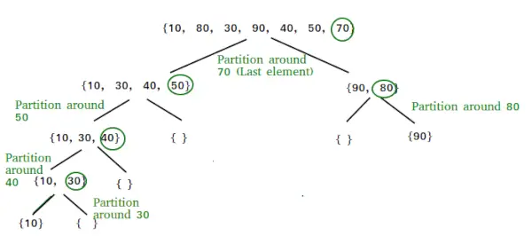
파티션 알고리즘
분할을 수행하는 방법에는 다음과 같이 여러 가지가 있을 수 있습니다. 의사 코드 CLRS 책에 제공된 방법을 채택합니다. 논리는 간단합니다. 가장 왼쪽 요소부터 시작하여 더 작은(또는 같은) 요소의 인덱스를 i로 추적합니다. 순회하는 동안 더 작은 요소를 찾으면 현재 요소를 arr[i]로 바꿉니다. 그렇지 않으면 현재 요소를 무시합니다.
피벗: end -= 1 # 시작과 끝이 서로 교차하지 않으면 # 시작과 끝의 숫자를 바꿉니다. if(start < end): array[start], array[end] = array[end], array[start] # Swap pivot element with element on end pointer. # This puts pivot on its correct sorted place. array[end], array[pivot_index] = array[pivot_index], array[end] # Returning end pointer to divide the array into 2 return end # The main function that implements QuickSort def quick_sort(start, end, array): if (start < end): # p is partitioning index, array[p] # is at right place p = partition(start, end, array) # Sort elements before partition # and after partition quick_sort(start, p - 1, array) quick_sort(p + 1, end, array) # Driver code array = [ 10, 7, 8, 9, 1, 5 ] quick_sort(0, len(array) - 1, array) print(f'Sorted array: {array}') 
산출
Sorted array: [1, 5, 7, 8, 9, 10]
시간 복잡도: O(n(logn))
쉘 정렬
쉘 정렬 주로 삽입 정렬의 변형입니다. 삽입 정렬에서는 요소를 한 위치 앞으로만 이동합니다. 요소를 훨씬 앞쪽으로 이동해야 할 경우 많은 이동이 필요합니다. shellSort의 아이디어는 멀리 있는 항목의 교환을 허용하는 것입니다. shellSort에서는 h의 큰 값에 대해 배열을 h 정렬합니다. h가 1이 될 때까지 h의 값을 계속 줄입니다. 모든 h의 모든 하위 목록이 h 정렬되었다고 합니다. 일 요소가 정렬되었습니다.
파이썬3 # Python3 program for implementation of Shell Sort def shellSort(arr): gap = len(arr) // 2 # initialize the gap while gap>0: i = 0 j = gap # 왼쪽에서 오른쪽으로 # j의 가능한 마지막 인덱스까지 배열을 확인합니다 while j < len(arr): if arr[i]>arr[j]: arr[i],arr[j] = arr[j],arr[i] i += 1 j += 1 # 이제 i번째 인덱스에서 왼쪽으로 돌아봅니다. # 값을 바꿉니다. 올바른 순서가 아닙니다. k = i 동안 k - 간격> -1: arr[k - 간격]> arr[k]인 경우: arr[k-gap],arr[k] = arr[k],arr[k-gap] k -= 1 gap //= 2 # 코드 확인을 위한 드라이버 arr2 = [12, 34, 54, 2, 3] print('input array:',arr2) shellSort(arr2) print('sorted array', arr2) 산출
input array: [12, 34, 54, 2, 3] sorted array [2, 3, 12, 34, 54]
시간 복잡도: 에 2 ).