Aquesta sèrie us introduirà a la creació de gràfics en Python amb Matplotlib, que és sens dubte la biblioteca de visualització de dades i gràfics més popular per a Python .
Instal·lació
La manera més senzilla d'instal·lar matplotlib és utilitzar pip. Escriviu la següent comanda al terminal:

pip install matplotlib 

O, podeu descarregar-lo des de aquí i instal·lar-lo manualment.

Hi ha diverses maneres de fer-ho a Python. aquí estem discutint alguns mètodes d'ús general per traçar matplotlib en Python. aquests són els següents.

• Traçant una línia
• Traçar dues o més línies a la mateixa trama
• Personalització de Parcel·les
• Gràfic de barres Matplotlib
• Traçant l'histograma Matplotlib
• Traçant Matplotlib Gràfic de dispersió
• Traçar un gràfic circular de Matplotlib
• Representació de corbes d'una equació donada

Traçant una línia

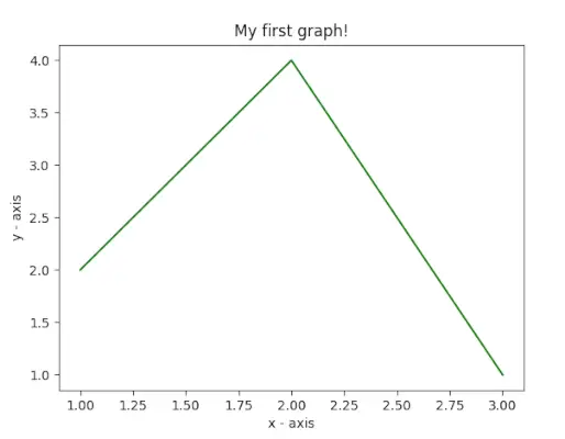
En aquest exemple, el codi utilitza Matplotlib per crear una traça de línies simple. Defineix valors x i y per als punts de dades, els representa mitjançant ` plt.plot() `, i etiqueta els eixos x i y amb `plt.xlabel()` i `plt.ylabel()`. La trama es titula El meu primer gràfic! utilitzant `plt.title()`. Finalment, el ` plt.show() La funció ` s'utilitza per mostrar el gràfic amb les dades especificades, les etiquetes dels eixos i el títol.

Python

# importing the required module> import> matplotlib.pyplot as plt> # x axis values> x> => [> 1> ,> 2> ,> 3> ]> # corresponding y axis values> y> => [> 2> ,> 4> ,> 1> ]> # plotting the points> plt.plot(x, y)> # naming the x axis> plt.xlabel(> 'x - axis'> )> # naming the y axis> plt.ylabel(> 'y - axis'> )> # giving a title to my graph> plt.title(> 'My first graph!'> )> # function to show the plot> plt.show()>

Sortida:

Traçar dues o més línies a la mateixa trama

En aquest exemple, el codi utilitza Matplotlib per crear un gràfic amb dues línies. Defineix dos conjunts de valors x i y per a cada línia i els representa mitjançant `plt.plot()`. Les línies s'etiqueten com a línia 1 i línia 2 amb el paràmetre 'etiqueta'. Els eixos s'etiqueten amb 'plt.xlabel()' i 'plt.ylabel()', i el gràfic es titula Dues línies en el mateix gràfic! amb `plt.title()`. La llegenda es mostra amb ` plt.legend() `, i la funció `plt.show()` s'utilitza per visualitzar el gràfic tant amb línies com amb etiquetes.

Python

import> matplotlib.pyplot as plt> # line 1 points> x1> => [> 1> ,> 2> ,> 3> ]> y1> => [> 2> ,> 4> ,> 1> ]> # plotting the line 1 points> plt.plot(x1, y1, label> => 'line 1'> )> # line 2 points> x2> => [> 1> ,> 2> ,> 3> ]> y2> => [> 4> ,> 1> ,> 3> ]> # plotting the line 2 points> plt.plot(x2, y2, label> => 'line 2'> )> # naming the x axis> plt.xlabel(> 'x - axis'> )> # naming the y axis> plt.ylabel(> 'y - axis'> )> # giving a title to my graph> plt.title(> 'Two lines on same graph!'> )> # show a legend on the plot> plt.legend()> # function to show the plot> plt.show()>

Sortida:

Personalització de Parcel·les

En aquest exemple, el codi utilitza Matplotlib per crear un traç de línies personalitzat. Defineix els valors x i y, i la trama té un estil amb una línia discontínua verda, un marcador circular blau per a cada punt i una mida del marcador de 12. Els límits de l'eix y s'estableixen en 1 i 8, i l'eix x els límits s'estableixen a 1 i 8 mitjançant `plt.ylim()` i `plt.xlim()`. Els eixos estan etiquetats amb `plt.xlabel()` i `plt.ylabel()`, i el gràfic es titula Algunes personalitzacions genials! amb `plt.title()`.

Python

import> matplotlib.pyplot as plt> # x axis values> x> => [> 1> ,> 2> ,> 3> ,> 4> ,> 5> ,> 6> ]> # corresponding y axis values> y> => [> 2> ,> 4> ,> 1> ,> 5> ,> 2> ,> 6> ]> # plotting the points> plt.plot(x, y, color> => 'green'> , linestyle> => 'dashed'> , linewidth> => 3> ,> > marker> => 'o'> , markerfacecolor> => 'blue'> , markersize> => 12> )> # setting x and y axis range> plt.ylim(> 1> ,> 8> )> plt.xlim(> 1> ,> 8> )> # naming the x axis> plt.xlabel(> 'x - axis'> )> # naming the y axis> plt.ylabel(> 'y - axis'> )> # giving a title to my graph> plt.title(> 'Some cool customizations!'> )> # function to show the plot> plt.show()>

Sortida:

Traçant Matplotlib Ús del diagrama de barres

En aquest exemple, el codi utilitza Matplotlib per crear un gràfic de barres. Defineix les coordenades x ('esquerra'), les altures de les barres ('altura') i les etiquetes de les barres ('tick_label'). La funció `plt.bar()` s'utilitza llavors per traçar el gràfic de barres amb paràmetres especificats com ara l'amplada de la barra, els colors i les etiquetes. Els eixos s'etiqueten amb `plt.xlabel()` i `plt.ylabel()`, i el gràfic es titula El meu gràfic de barres! utilitzant `plt.title()`.

Python

import> matplotlib.pyplot as plt> # x-coordinates of left sides of bars> left> => [> 1> ,> 2> ,> 3> ,> 4> ,> 5> ]> # heights of bars> height> => [> 10> ,> 24> ,> 36> ,> 40> ,> 5> ]> # labels for bars> tick_label> => [> 'one'> ,> 'two'> ,> 'three'> ,> 'four'> ,> 'five'> ]> # plotting a bar chart> plt.bar(left, height, tick_label> => tick_label,> > width> => 0.8> , color> => [> 'red'> ,> 'green'> ])> # naming the x-axis> plt.xlabel(> 'x - axis'> )> # naming the y-axis> plt.ylabel(> 'y - axis'> )> # plot title> plt.title(> 'My bar chart!'> )> # function to show the plot> plt.show()>

Sortida:

Traçant Matplotlib Ús de l'histograma

En aquest exemple, el codi utilitza Matplotlib per crear un histograma. Defineix una llista de freqüències d'edat ( ages> ), estableix l'interval de valors de 0 a 100 i especifica el nombre de safates com a 10. plt.hist()> A continuació, s'utilitza la funció per traçar l'histograma amb les dades i el format proporcionats, inclosos el color, el tipus d'histograma i l'amplada de la barra. Els eixos estan etiquetats amb plt.xlabel()> i plt.ylabel()> , i el gràfic es titula El meu histograma fent servir plt.title()> .

Python

import> matplotlib.pyplot as plt> # frequencies> ages> => [> 2> ,> 5> ,> 70> ,> 40> ,> 30> ,> 45> ,> 50> ,> 45> ,> 43> ,> 40> ,> 44> ,> > 60> ,> 7> ,> 13> ,> 57> ,> 18> ,> 90> ,> 77> ,> 32> ,> 21> ,> 20> ,> 40> ]> # setting the ranges and no. of intervals> range> => (> 0> ,> 100> )> bins> => 10> # plotting a histogram> plt.hist(ages, bins,> range> , color> => 'green'> ,> > histtype> => 'bar'> , rwidth> => 0.8> )> # x-axis label> plt.xlabel(> 'age'> )> # frequency label> plt.ylabel(> 'No. of people'> )> # plot title> plt.title(> 'My histogram'> )> # function to show the plot> plt.show()>

Sortida:

Traçant Matplotlib Ús del diagrama de dispersió

En aquest exemple, el codi utilitza Matplotlib per crear un diagrama de dispersió. Defineix els valors de x i y i els representa com a punts de dispersió amb marcadors d'asterisc verd (`*`) de mida 30. Els eixos s'etiqueten amb `plt.xlabel()` i `plt.ylabel()`, i la trama porta el títol La meva trama de dispersió! utilitzant `plt.title()`. La llegenda es mostra amb les estrelles de l'etiqueta utilitzant `plt.legend()`, i el diagrama de dispersió resultant es mostra amb `plt.show()`.

Python

import> matplotlib.pyplot as plt> # x-axis values> x> => [> 1> ,> 2> ,> 3> ,> 4> ,> 5> ,> 6> ,> 7> ,> 8> ,> 9> ,> 10> ]> # y-axis values> y> => [> 2> ,> 4> ,> 5> ,> 7> ,> 6> ,> 8> ,> 9> ,> 11> ,> 12> ,> 12> ]> # plotting points as a scatter plot> plt.scatter(x, y, label> => 'stars'> , color> => 'green'> ,> > marker> => '*'> , s> => 30> )> # x-axis label> plt.xlabel(> 'x - axis'> )> # frequency label> plt.ylabel(> 'y - axis'> )> # plot title> plt.title(> 'My scatter plot!'> )> # showing legend> plt.legend()> # function to show the plot> plt.show()>

Sortida:

Traçant Matplotlib Ús de gràfic circular

En aquest exemple, el codi utilitza Matplotlib per crear un gràfic circular. Defineix etiquetes per a diferents activitats ('activitats'), la part coberta per cada etiqueta ('slices') i colors per a cada etiqueta ('colors'). Aleshores, la funció `plt.pie()` s'utilitza per dibuixar el gràfic circular amb diverses opcions de format, com ara l'angle inicial, l'ombra, l'explosió per a un sector específic, el radi i l'autopct per a la visualització del percentatge. La llegenda s'afegeix amb `plt.legend()`, i el gràfic de sectors resultant es mostra amb `plt.show()`.

Python

import> matplotlib.pyplot as plt> # defining labels> activities> => [> 'eat'> ,> 'sleep'> ,> 'work'> ,> 'play'> ]> # portion covered by each label> slices> => [> 3> ,> 7> ,> 8> ,> 6> ]> # color for each label> colors> => [> 'r'> ,> 'y'> ,> 'g'> ,> 'b'> ]> # plotting the pie chart> plt.pie(slices, labels> => activities, colors> => colors,> > startangle> => 90> , shadow> => True> , explode> => (> 0> ,> 0> ,> 0.1> ,> 0> ),> > radius> => 1.2> , autopct> => '%1.1f%%'> )> # plotting legend> plt.legend()> # showing the plot> plt.show()>

La sortida del programa anterior té aquest aspecte:

Representació de corbes d'una equació donada

En aquest exemple, el codi utilitza Matplotlib i NumPy per crear una gràfica d'ona sinusoïdal. Genera coordenades x de 0 a 2π en increments de 0,1 utilitzant 'np.arange()' i calcula les coordenades y corresponents prenent el sinus de cada valor x amb 'np.sin()'. A continuació, els punts es representen mitjançant `plt.plot()`, donant lloc a una ona sinusoïdal. Finalment, la funció `plt.show()` s'utilitza per mostrar la gràfica d'ona sinusoïdal.

Python

# importing the required modules> import> matplotlib.pyplot as plt> import> numpy as np> # setting the x - coordinates> x> => np.arange(> 0> ,> 2> *> (np.pi),> 0.1> )> # setting the corresponding y - coordinates> y> => np.sin(x)> # plotting the points> plt.plot(x, y)> # function to show the plot> plt.show()>

Sortida:

Així, en aquesta part, hem parlat de diversos tipus de trames que podem crear a matplotlib. Hi ha més trames que no s'han cobert, però les més significatives es comenten aquí:

• Traçat gràfic en Python | Set 2
• Traçat gràfic en Python | Set 3

Si t'agrada techcodeview.com i vols contribuir, també pots escriure un article mitjançant write.techcodeview.com o enviar el teu article a [email protected]
Si us plau, escriviu comentaris si trobeu alguna cosa incorrecta o voleu compartir més informació sobre el tema tractat anteriorment.